1 Introduction
The capability of R to do symbolic mathematics is enhanced by the
reticulate (Ushey et al. 2020) and caracas (Andersen and Højsgaard 2021)
packages.
The reticulate package allows R users to make use of various Python
libraries, such as the symbolic mathematics package SymPy, which is
the workhorse behind symbolic mathematics in this connection.
However, the reticulate package does require that the users are
somewhat familiar with Python syntax. The caracas package, on the
other hand, provides an interface to reticulate that conforms fully to
the existing R syntax. In short form, caracas provides the
following:
Mathematical tools like equation solving, summation, limits, symbolic linear algebra in R syntax and formatting of tex output.
Symbolic mathematics can easily be combined with data which is helpful in e.g. numerical optimization.
In this paper we will illustrate the use of the caracas package
(version 2.1.0) in connection with teaching mathematics and statistics
and how students can benefit benefit from bridging computer algebra and data
via R.
Focus is on: 1) treating statistical models symbolically, 2)
bridging the gap between symbolic mathematics and numerical
computations and 3) preparing teaching material in a reproducible
framework
(provided by, e.g. rmarkdown and Quarto; Allaire et al. (2021); Xie et al. (2018); Xie et al. (2020); Allaire et al. (2022))
.
The caracas package is available from CRAN. Several vignettes
illustrating caracas are provided with the package and they are also
available online together with the help pages, see
https://r-cas.github.io/caracas/. The development
version of caracas is available at
https://github.com/r-cas/caracas.
The paper is organized in the following sections: The section
Introducing caracas briefly introduces
the caracas package and its syntax, and
relates caracas to SymPy via reticulate.
The section Statistics examples presents a sample of statistical models
where we believe that a
symbolic treatment can enhance purely numerical computations.
In the section Further topics we
demonstrate further aspects of caracas, including how caracas can be
used in connection with preparing texts, e.g. teaching material and
working documents.
The section Hands-on activities
contains suggestions about hands-on activities, e.g. for students.
The last section Discussion contains a discussion of the
paper.
1.1 Installation
The caracas package is available on CRAN and can be installed as usual with install.packages('caracas').
Please ensure that you have SymPy installed, or else install it:
if (!caracas::has_sympy()) {
  caracas::install_sympy()
}
The caracas package relies on the reticulate package to run Python code.
Thus, if you wish to configure your Python environment, you need to
first load reticulate, then configure the Python environment, and at
last load caracas.
The Python environment can be configured as
in reticulate’s “Python Version Configuration” vignette.
Again, configuring the Python environment needs to be done before
loading caracas.
Please find further details in reticulate’s documentation.
2 Introducing caracas
Here we introduce key concepts and show functionality subsequently
needed in the section Statistics examples.
We will demonstrate both caracas and
contrast this with using reticulate directly.
2.1 Symbols
A caracas symbol is a list with a pyobj slot and the class
caracas_symbol. The pyobj is a Python object (often a SymPy
object). As such, a caracas symbol (in R) provides a handle to a
Python object. In the design of caracas we have tried to make
this distinction something the user should not be concerned with, but
it is worthwhile being aware of the distinction. Whenever we refer to
a symbol we mean a caracas symbol. Two functions that create
symbols are def_sym() and as_sym(); these and other functions that
create symbols will be illustrated below.
2.2 Linear algebra
We create a symbolic matrix (a caracas symbol) from an R object and
a symbolic vector (a caracas symbol) directly. A vector is a
one-column matrix which is printed as its transpose to save
space. Matrix products are computed using the %*% operator:
Here we make use of the fact that caracas is tightly integrated with R
which has a toeplitz() function that can be used.
Similarly, caracas offers matrix_sym() and
vector_sym() for generating general matrix and vector objects.
The object M is
Mc: [[a, b],
[b, a]]The LaTeX rendering using the tex() function of the symbols
above are (refer to section Further topics):
\[\begin{equation} M = \left[\begin{matrix}a & b\\b & a\end{matrix}\right]; \; v = \left[\begin{matrix}v_{1}\\v_{2}\end{matrix}\right]; \; y = \left[\begin{matrix}a v_{1} + b v_{2}\\a v_{2} + b v_{1}\end{matrix}\right]; \; M^{-1} = \left[\begin{matrix}\frac{a}{a^{2} - b^{2}} & - \frac{b}{a^{2} - b^{2}}\\- \frac{b}{a^{2} - b^{2}} & \frac{a}{a^{2} - b^{2}}\end{matrix}\right]; \; w = \left[\begin{matrix}v_{1}\\v_{2}\end{matrix}\right] . \end{equation}\]
Symbols can be substituted with other symbols or with numerical values
using subs().
\[\begin{equation} M2 = \left[\begin{matrix}a & a^{2}\\a^{2} & a\end{matrix}\right]; \quad M3 = \left[\begin{matrix}2 & 4\\4 & 2\end{matrix}\right]. \end{equation}\]
2.3 Linear algebra - using reticulate
The reticulate package already enables SymPy from within R,
but does not use standard R syntax for many operations (e.g. matrix multiplication),
and certain operations are more complicated than the R counterparts
(e.g. replacing elements in a matrix and constructing R expressions).
As illustration, the previous linear algebra example can also be done using reticulate:
library(reticulate)
sympy <- import("sympy")
M_ <- sympy$Matrix(list(c("a_", "b_"), c("b_", "a_")))
v_ <- sympy$Matrix(list("v1_", "v2_"))
y_ <- M_ * v_
w_ <- M_$inv() * y_
sympy$simplify(w_)
Matrix([
[v1_],
[v2_]])This shows that it is possible to do the same linear algebra example
using only reticulate,
but it requires using non-standard R syntax (for
example, using * for matrix multiplication instead of %*%).
2.4 Functionality and R syntax provided by caracas
In caracas we use R syntax:
The code correspondence between reticulate and caracas shows
that the same can be achieved with reticulate. However, it can be argued that
the syntax is more involved, at least for users only familiar with R. Note in particular that
Python’s “object-oriented” syntax can make code harder to read due to
having to call methods with $:
Notice that SymPy uses 0-based indexing (as Python does), whereas
caracas uses 1-based indexing (as R does). Furthermore, indexing
has to be done using explicit integers
so above we write 1L (an integer) rather than simply 1
(a numeric).
We have already shown that caracas can coerce R matrices to
symbols. Additionally, caracas provides various convenience
functions:
M <- matrix_sym(2, 2, entry = "sigma")
D <- matrix_sym_diag(2, entry = "d")
S <- matrix_sym_symmetric(2, entry = "s")
E <- eye_sym(2, 2)
J <- ones_sym(2, 2)
b <- vector_sym(2, entry = "b")
\[\begin{equation} M = \left[\begin{matrix}\sigma_{11} & \sigma_{12}\\\sigma_{21} & \sigma_{22}\end{matrix}\right]; D = \left[\begin{matrix}d_{1} & 0\\0 & d_{2}\end{matrix}\right]; S = \left[\begin{matrix}s_{11} & s_{21}\\s_{21} & s_{22}\end{matrix}\right]; E = \left[\begin{matrix}1 & 0\\0 & 1\end{matrix}\right]; J = \left[\begin{matrix}1 & 1\\1 & 1\end{matrix}\right]; b = \left[\begin{matrix}b_{1}\\b_{2}\end{matrix}\right] \end{equation}\]
A caracas symbol can be turned into an R function for subsequent
numerical evaluation using as_func() or into an R expression using as_expr():
as_func(M)function (sigma11, sigma12, sigma21, sigma22)
{
matrix(c(sigma11, sigma21, sigma12, sigma22), nrow = 2)
}
<environment: 0x10f0379a8>as_expr(M)expression(matrix(c(sigma11, sigma21, sigma12, sigma22), nrow = 2))2.5 Algebra and calculus
We can define a polynomial \(p\) in the variable \(x\). This is done by
defining a caracas symbol x and subsequently a caracas
polynomial p in x (notice that p gets automatically coerced into
a symbol as well, because p is defined in terms of the symbol x):
def_sym(x)
p <- 1 - x^2 + x^3 + x^4/4 - 3 * x^5 / 5 + x^6 / 6
The function def_sym() creates the symbol x.
Alternatively, x <- as_sym("x") can be used,
but it has the drawback that you could also write y <- as_sym("x").
We investigate p further by finding the first and second derivatives of p, i.e. the gradient and Hessian of
p.
Notice here that some functions have a postfix underscore as a simple
way of distinguishing them from R functions with a different
meaning. Thus, here the function factor_() factorizes the polynomial
which shows that the stationary points are
\(-1\), \(0\), \(1\) and \(2\):
\[\begin{equation} \texttt{g} = x^{5} - 3 x^{4} + x^{3} + 3 x^{2} - 2 x; \quad \texttt{g2} = x \left(x - 2\right) \left(x - 1\right)^{2} \left(x + 1\right). \end{equation}\]
In a more general setting we can find the stationary points by equating the gradient to zero:
The output sol is a list of solutions in which each solution is a list of caracas symbols.
sol <- solve_sys(lhs = g, rhs = 0, vars = x)
sol
x = -1
x = 0
x = 1
x = 2Notice that solve_sys also works with complex solutions:
solve_sys(lhs = x^2 + 1, rhs = 0, vars = x)x = -1i
x = 1iAs noted before, a caracas symbol can be coerced to an R expression
using as_expr(). This can be used to get the roots of g
(the stationary points) above as an R object.
The sign of the second derivative in the stationary points can be obtained
by coercing the second derivative symbol to a function:
The sign of the second derivative in the stationary points shows that \(-1\) and \(2\) are local minima, \(0\) is a local maximum and \(1\) is an inflection point. The polynomial, the first derivative and the second derivative are shown in Fig. 1. The stationary points, \(-1, 0, 1, 2\), are indicated in the plots.
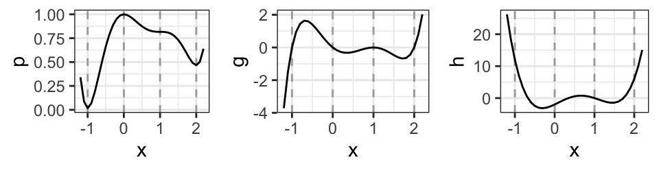
Figure 1: Left: A polynomial. Center: First derivative (the gradient). Right: Second derivative (the Hessian).
3 Statistics examples
In this section we examine larger statistical examples and
demonstrate how caracas can help improve understanding of the models.
3.1 Example: Linear models
While the matrix form of linear models is quite clear and concise, it can also be argued that matrix algebra obscures what is being computed. Numerical examples are useful for some aspects of the computations but not for others. In this respect symbolic computations can be enlightening.
Consider a two-way analysis of variance (ANOVA) with one observation per group, see Table 1.
| \(y_{11}\) | \(y_{12}\) |
| \(y_{21}\) | \(y_{22}\) |
Previously, it was demonstrated that a symbolic
vector could be defined with the vector_sym() function.
Another way to specify a symbolic vector with explicit elements is
by using as_sym():
y  <- as_sym(c("y_11", "y_21", "y_12", "y_22"))
dat <- expand.grid(r = factor(1:2), s = factor(1:2))
X <- model.matrix(~ r + s, data = dat) |> as_sym()
b <- vector_sym(ncol(X), "b")
mu <- X %*% b
For the specific model we have random variables \(y=(y_{ij})\). All \(y_{ij}\)s are assumed independent and \(y_{ij}\sim N(\mu_{ij}, v)\). The corresponding mean vector \(\mu\) has the form given below:
\[\begin{equation} y = \left[\begin{matrix}y_{11}\\y_{21}\\y_{12}\\y_{22}\end{matrix}\right]; \quad X=\left[\begin{matrix}1 & . & .\\1 & 1 & .\\1 & . & 1\\1 & 1 & 1\end{matrix}\right]; \quad b=\left[\begin{matrix}b_{1}\\b_{2}\\b_{3}\end{matrix}\right]; \quad \mu = X b = \left[\begin{matrix}b_{1}\\b_{1} + b_{2}\\b_{1} + b_{3}\\b_{1} + b_{2} + b_{3}\end{matrix}\right] . \end{equation}\]
Above and elsewhere, dots represent zero. The least squares estimate of \(b\) is the vector \(\hat{b}\) that minimizes \(||y-X b||^2\) which leads to the normal equations \((X^\top X)b = X^\top y\) to be solved. If \(X\) has full rank, the unique solution to the normal equations is \(\hat{b} = (X^\top X)^{-1} X^\top y\). Hence the estimated mean vector is \(\hat \mu = X\hat{b}=X(X^\top X)^{-1} X^\top y\). Symbolic computations are not needed for quantities involving only the model matrix \(X\), but when it comes to computations involving \(y\), a symbolic treatment of \(y\) is useful:
\[\begin{align} X^\top y &= \left[\begin{matrix}y_{11} + y_{12} + y_{21} + y_{22}\\y_{21} + y_{22}\\y_{12} + y_{22}\end{matrix}\right]; \quad \quad \hat{b} = \frac{1}{2} \left[\begin{matrix}\frac{3 y_{11}}{2} + \frac{y_{12}}{2} + \frac{y_{21}}{2} - \frac{y_{22}}{2}\\- y_{11} - y_{12} + y_{21} + y_{22}\\- y_{11} + y_{12} - y_{21} + y_{22}\end{matrix}\right]. \end{align}\]
Hence \(X^\top y\) (a sufficient reduction of data if the variance is known) consists of the sum of all observations, the sum of observations in the second row and the sum of observations in the second column. For \(\hat{b}\), the second component is, apart from a scaling, the sum of the second row minus the sum of the first row. Likewise, the third component is the sum of the second column minus the sum of the first column. Hence, for example the second component of \(\hat{b}\) is the difference in mean between the first and second column in Table 1.
3.2 Example: Logistic regression
In the following we go through details of the logistic regression model, for a classical description see e.g. McCullagh and Nelder (1989) for a classical description.
As an example, consider the budworm data from the doBy package (Højsgaard and Halekoh 2023).
The data shows the number of killed moth tobacco budworm
. Batches of 20 moths of each sex were
exposed for three days to the pyrethroid and the number in each batch
that were dead or knocked down was recorded.
Below we focus only on male budworms and the mortality is illustrated
in Figure 2 (produced with ggplot2; Wickham (2016)). The \(y\)-axis shows the empirical
logits, i.e. \(\log((\texttt{ndead} + 0.5)/(\texttt{ntotal}-\texttt{ndead} + 0.5))\). The figure suggests that log odds of dying grows linearly with log dose.
   sex dose ndead ntotal
1 male    1     1     20
2 male    2     4     20
3 male    4     9     20
4 male    8    13     20
5 male   16    18     20
6 male   32    20     20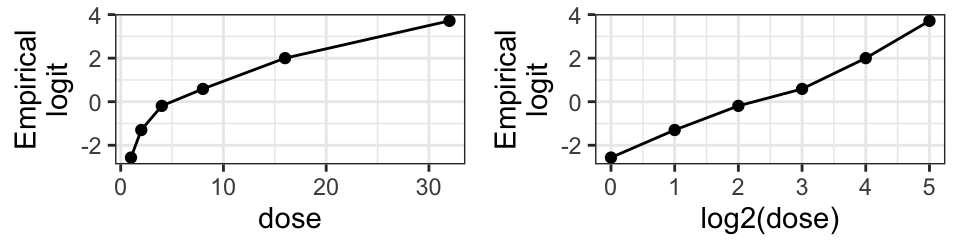
Figure 2: Insecticide mortality of the moth tobacco budworm.
Observables are binomially distributed, \(y_i \sim \text{bin}(p_i, n_i)\). The probability \(p_i\) is connected to a \(q\)-vector of covariates \(x_i=(x_{i1}, \dots, x_{iq})\) and a \(q\)-vector of regression coefficients \(b=(b_1, \dots, b_q)\) as follows: The term \(s_i = x_i \cdot b\) is denoted the . The probability \(p_i\) can be linked to \(s_i\) in different ways, but the most commonly employed is via the which is \(\text{logit}(p_i) = \log(p_i/(1-p_i))\) so here \(\text{logit}(p_i) = s_i\). Based on Figure 2, we consider the specific model with \(s_i = b_1 + b_2 \log2(dose_i)\). For later use, we define the data matrix below:
DM <- cbind(model.matrix(~log2(dose), data=bud),
            bud[, c("ndead", "ntotal")])  |> as.matrix()
DM |> head(3)
(Intercept) log2(dose) ndead ntotal
1 1 0 1 20
2 1 1 4 20
3 1 2 9 20Each component of the likelihood
The log-likelihood is \(\log L=\sum_i y_i \log(p_i) + (n_i-y_i) \log(1-p_i) = \sum_i \log L_i\), say. Consider the contribution to the total log-likelihood from the \(i\)th observation which is \(\log L_i = l_i = y_i \log(p_i) + (n_i-y_i) \log(1-p_i)\). Since we are focusing on one observation only, we shall ignore the subscript \(i\) in this section. First notice that with \(s = \log(p/(1-p))\) we can find \(p\) as a function of \(s\) as:
\[\begin{equation} \texttt{p\_s} = \frac{e^{s}}{e^{s} + 1} \end{equation}\]
Next, find the likelihood as a function of \(p\), as a function of \(s\)
and as a function of \(b\). The underscore in logLb_ and elsewhere
indicates that this expression is defined in terms of other
symbols. The log-likelihood can be maximized using e.g. Newton-Raphson
(see e.g. Nocedal and Wright (2006)) and in this connection we need the score function,
\(S\), and the Hessian, \(H\):
def_sym(y, n)
b  <- vector_sym(2, "b")
x  <- vector_sym(2, "x")
logLp_ <- y * log(p) + (n - y) * log(1 - p) # logL as fn of p
s_b <- sum(x * b)                           # s as fn of b
p_b <- subs(p_s, s, s_b)                    # p as fn of b
logLb_ <- subs(logLp_, p, p_b)              # logL as fn of b
Sb_ <- score(logLb_, b) |> simplify()
Hb_ <- hessian(logLb_, b) |> simplify()
\[\begin{align} \texttt{p\_b} &= \frac{e^{b_{1} x_{1} + b_{2} x_{2}}}{e^{b_{1} x_{1} + b_{2} x_{2}} + 1}; \\ \texttt{logLb}\_ &= y \log{\left(\frac{e^{b_{1} x_{1} + b_{2} x_{2}}}{e^{b_{1} x_{1} + b_{2} x_{2}} + 1} \right)} + \left(n - y\right) \log{\left(1 - \frac{e^{b_{1} x_{1} + b_{2} x_{2}}}{e^{b_{1} x_{1} + b_{2} x_{2}} + 1} \right)}; \\ \texttt{Sb}\_ &= \left[\begin{matrix}\frac{x_{1} \left(- n e^{b_{1} x_{1} + b_{2} x_{2}} + y e^{b_{1} x_{1} + b_{2} x_{2}} + y\right)}{e^{b_{1} x_{1} + b_{2} x_{2}} + 1}\\\frac{x_{2} \left(- n e^{b_{1} x_{1} + b_{2} x_{2}} + y e^{b_{1} x_{1} + b_{2} x_{2}} + y\right)}{e^{b_{1} x_{1} + b_{2} x_{2}} + 1}\end{matrix}\right]; \\ \texttt{Hb}\_ &= \left[\begin{matrix}- \frac{n x_{1}^{2} e^{b_{1} x_{1} + b_{2} x_{2}}}{2 e^{b_{1} x_{1} + b_{2} x_{2}} + e^{2 b_{1} x_{1} + 2 b_{2} x_{2}} + 1} & - \frac{n x_{1} x_{2} e^{b_{1} x_{1} + b_{2} x_{2}}}{2 e^{b_{1} x_{1} + b_{2} x_{2}} + e^{2 b_{1} x_{1} + 2 b_{2} x_{2}} + 1}\\- \frac{n x_{1} x_{2} e^{b_{1} x_{1} + b_{2} x_{2}}}{2 e^{b_{1} x_{1} + b_{2} x_{2}} + e^{2 b_{1} x_{1} + 2 b_{2} x_{2}} + 1} & - \frac{n x_{2}^{2} e^{b_{1} x_{1} + b_{2} x_{2}}}{2 e^{b_{1} x_{1} + b_{2} x_{2}} + e^{2 b_{1} x_{1} + 2 b_{2} x_{2}} + 1}\end{matrix}\right] . \end{align}\]
There are some possible approaches before maximizing the total log likelihood. One is to insert data case by case into the symbolic log likelihood:
nms <- c("x1", "x2", "y", "n")
DM_lst <- doBy::split_byrow(DM)
logLb_lst <- lapply(DM_lst, function(vls) {
    subs(logLb_, nms, vls)
})
For example, the contribution from the third observation to the total log likelihood is:
\[\begin{align} \texttt{logLb\_lst[[3]]} &= 9 \log{\left(\frac{e^{b_{1} + 2 b_{2}}}{e^{b_{1} + 2 b_{2}} + 1} \right)} + 11 \log{\left(1 - \frac{e^{b_{1} + 2 b_{2}}}{e^{b_{1} + 2 b_{2}} + 1} \right)}. \end{align}\]
The full likelihood can be maximized either e.g. using SymPy (not pursued here) or by converting the sum to an R function which can be maximized using one of R’s internal optimization procedures:
logLb_tot <- Reduce(`+`, logLb_lst)
logLb_fn  <- as_func(logLb_tot, vec_arg = TRUE)
opt <- optim(c(b1 = 0, b2 = 0), logLb_fn,
              control = list(fnscale = -1), hessian = TRUE)
opt$par
b1 b2
-2.82 1.26 The same model can be fitted e.g. using R’s glm() function as follows:
(Intercept)  log2(dose)
      -2.82        1.26
The total likelihood symbolically
We conclude this section by illustrating that the log-likelihood for the entire dataset can be constructed in a few steps (output is omitted to save space):
N <- 6; q <- 2
X <- matrix_sym(N, q, "x")
n <- vector_sym(N, "n")
y <- vector_sym(N, "y")
p <- vector_sym(N, "p")
s <- vector_sym(N, "s")
b <- vector_sym(q, "b")
\[\begin{equation} X=\left[\begin{matrix}x_{11} & x_{12}\\x_{21} & x_{22}\\x_{31} & x_{32}\\x_{41} & x_{42}\\x_{51} & x_{52}\\x_{61} & x_{62}\end{matrix}\right]; \quad n=\left[\begin{matrix}n_{1}\\n_{2}\\n_{3}\\n_{4}\\n_{5}\\n_{6}\end{matrix}\right]; \quad y=\left[\begin{matrix}y_{1}\\y_{2}\\y_{3}\\y_{4}\\y_{5}\\y_{6}\end{matrix}\right] . \end{equation}\]
The symbolic computations are as follows: We express the linear predictor \(s\) as function of the regression coefficients \(b\) and express the probability \(p\) as function of the linear predictor:
Next step could be to go from symbolic to numerical computations by inserting numerical values. From here, one may proceed by computing the score function and the Hessian matrix and solve the score equation, using e.g. Newton-Raphson. Alternatively, one might create an R function based on the log-likelihood, and maximize this function using one of R’s optimization methods (see the example in the previous section):
logLb <- subs(logLb_, cbind(X, y, n), DM)
logLb_fn <- as_func(logLb, vec_arg = TRUE)
opt <- optim(c(b1 = 0, b2 = 0), logLb_fn,
              control = list(fnscale = -1), hessian = TRUE)
opt$par
b1 b2
-2.82 1.26 3.3 Example: Constrained maximum likelihood
In this section we illustrate constrained optimization using Lagrange multipliers. This is demonstrated for the independence model for a two-way contingency table. Consider a \(2 \times 2\) contingency table with cell counts \(y_{ij}\) and cell probabilities \(p_{ij}\) for \(i=1,2\) and \(j=1,2\), where \(i\) refers to row and \(j\) to column as illustrated in Table 1.
Under multinomial sampling, the log likelihood is
\[\begin{equation} l = \log L = \sum_{ij} y_{ij} \log(p_{ij}). \end{equation}\]
Under the assumption of independence between rows and columns, the cell probabilities have the form, (see e.g. Højsgaard et al. (2012), p. 32)
\[\begin{equation} p_{ij}=u \cdot r_i \cdot s_j. \end{equation}\]
To make the parameters \((u, r_i, s_j)\) identifiable, constraints
must be imposed. One possibility is to require that \(r_1=s_1=1\). The
task is then to estimate \(u\), \(r_2\), \(s_2\) by maximizing the log likelihood
under the constraint that \(\sum_{ij} p_{ij} = 1\). These constraints
can be
imposed using a Lagrange multiplier where we solve the
unconstrained optimization problem \(\max_p Lag(p)\) where
\[\begin{align}
Lag(p) &= -l(p) + \lambda g(p) \quad \text{under the constraint that} \\
g(p) &= \sum_{ij} p_{ij} - 1 = 0 ,
\end{align}\]
where \(\lambda\) is a Lagrange multiplier.
The likelihood equations can be found in closed-form.
In SymPy, lambda is a reserved symbol so it is denoted by an postfixed underscore below:
def_sym(u, r2, s2, lambda_)
y  <- as_sym(c("y_11", "y_21", "y_12", "y_22"))
p  <- as_sym(c("u", "u*r2", "u*s2", "u*r2*s2"))
logL <- sum(y * log(p))
Lag  <- -logL + lambda_ * (sum(p) - 1)
vars <- list(u, r2, s2, lambda_)
gLag <- der(Lag, vars)
sol  <- solve_sys(gLag, vars)
print(sol, method = "ascii")
Solution 1:
lambda_ = y_11 + y_12 + y_21 + y_22
r2 = (y_21 + y_22)/(y_11 + y_12)
s2 = (y_12 + y_22)/(y_11 + y_21)
u = (y_11 + y_12)*(y_11 + y_21)/(y_11 + y_12 + y_21 + y_22)^2 sol <- sol[[1]]There is only one critical point. The fitted cell probabilities \(\hat p_{ij}\) are:
\[\begin{equation} \hat p = \frac{1}{\left(y_{11} + y_{12} + y_{21} + y_{22}\right)^{2}} \left[\begin{matrix}\left(y_{11} + y_{12}\right) \left(y_{11} + y_{21}\right) & \left(y_{11} + y_{12}\right) \left(y_{12} + y_{22}\right)\\\left(y_{11} + y_{21}\right) \left(y_{21} + y_{22}\right) & \left(y_{12} + y_{22}\right) \left(y_{21} + y_{22}\right)\end{matrix}\right] \end{equation}\]
To verify that the maximum likelihood estimate has been found, we compute the Hessian matrix which is negative definite (the Hessian matrix is diagonal so the eigenvalues are the diagonal entries and these are all negative), output omitted:
3.4 Example: An auto regression model
Symbolic computations
In this section we study the auto regressive model of order \(1\) (an AR(1) model, see e.g. Shumway and Stoffer (2016), p. 75): Consider random variables \(x_1, x_2, \dots, x_n\) following a stationary zero mean AR(1) process:
\[\begin{equation} x_i = a x_{i-1} + e_i; \quad i=2, \dots, n, \tag{1} \end{equation}\]
where \(e_i \sim N(0, v)\) and all independent and with constant variance \(v\). The marginal distribution of \(x_1\) is also assumed normal, and for the process to be stationary we must have that the variance \(\mathbf{Var}(x_1) = v / (1-a^2)\). Hence we can write \(x_1 = \frac 1 {\sqrt{1-a^2}} e_1\).
For simplicity of exposition, we set \(n=4\) such that \(e=(e_1, \dots, e_4)\) and \(x=(x_1, \dots x_4)\). Hence \(e \sim N(0, v I)\). Isolating error terms in (1) gives
\[\begin{equation} e= \left[\begin{matrix}e_{1}\\e_{2}\\e_{3}\\e_{4}\end{matrix}\right] = \left[\begin{matrix}\sqrt{1 - a^{2}} & . & . & .\\- a & 1 & . & .\\. & - a & 1 & .\\. & . & - a & 1\end{matrix}\right] \left[\begin{matrix}x_{1}\\x_{2}\\x_{3}\\x_{4}\end{matrix}\right] = L x . \end{equation}\]
Since \(\mathbf{Var}(e)=v I\) we have \(\mathbf{Var}(e)=v I=L \mathbf{Var}(x) L^\top\) so the covariance matrix of \(x\) is \(V=\mathbf{Var}(x) = v L^{-1} \left (L^{-1} \right )^\top\) while the concentration matrix (the inverse covariance matrix) is \(K=v^{-1}L^\top L\):
def_sym(a, v)
n <- 4
L <- diff_mat(n, "-a") # The difference matrix, L, shown above
L[1, 1] <- sqrt(1 - a^2)
Linv <- solve(L)
K <- crossprod_(L) / v
V <- tcrossprod_(Linv) * v
\[\begin{align} L^{-1} &= \left[\begin{matrix}\frac{1}{\sqrt{1 - a^{2}}} & . & . & .\\\frac{a}{\sqrt{1 - a^{2}}} & 1 & . & .\\\frac{a^{2}}{\sqrt{1 - a^{2}}} & a & 1 & .\\\frac{a^{3}}{\sqrt{1 - a^{2}}} & a^{2} & a & 1\end{matrix}\right] ; \\ K &= \frac{1}{v} \left[\begin{matrix}1 & - a & 0 & 0\\- a & a^{2} + 1 & - a & 0\\0 & - a & a^{2} + 1 & - a\\0 & 0 & - a & 1\end{matrix}\right] ; \\ V &= \frac{v}{a^{2} - 1} \left[\begin{matrix}-1 & - a & - a^{2} & - a^{3}\\- a & -1 & - a & - a^{2}\\- a^{2} & - a & -1 & - a\\- a^{3} & - a^{2} & - a & -1\end{matrix}\right] . \end{align}\]
The zeros in the concentration matrix \(K\) implies a conditional independence restriction: If the \(ij\)th element of a concentration matrix is zero then \(x_i\) and \(x_j\) are conditionally independent given all other variables (see e.g. Højsgaard et al. (2012), p. 84 for details).
Next, we take the step from symbolic computations to numerical evaluations. The joint distribution of \(x\) is multivariate normal distribution, \(x\sim N(0, K^{-1})\). Let \(W=x x^\top\) denote the matrix of (cross) products. The log-likelihood is therefore (ignoring additive constants)
\[\begin{equation} \log L = \frac n 2 (\log \mathbf{det}(K) - x^\top K x) = \frac n 2 (\log \mathbf{det}(K) - \mathbf{tr}(K W)), \end{equation}\]
where we note that \(\mathbf{tr}(KW)\) is the sum of the elementwise products of \(K\) and \(W\) since both matrices are symmetric. Ignoring the constant \(\frac n 2\), this can be written symbolically to obtain the expression in this particular case:
\[\begin{equation} \log L = \log{\left(- \frac{a^{2}}{v^{4}} + \frac{1}{v^{4}} \right)} - \frac{- 2 a x_{1} x_{2} - 2 a x_{2} x_{3} - 2 a x_{3} x_{4} + x_{1}^{2} + x_{2}^{2} \left(a^{2} + 1\right) + x_{3}^{2} \left(a^{2} + 1\right) + x_{4}^{2}}{v} . \end{equation}\]
Numerical evaluation
Next we illustrate how bridge the gap from symbolic computations to numerical computations based on a dataset: For a specific data vector we get:
\[\begin{equation} \log L = \log{\left(- \frac{a^{2}}{v^{4}} + \frac{1}{v^{4}} \right)} - \frac{0.97 a^{2} + 0.9 a + 0.98}{v} . \end{equation}\]
We can use R for numerical maximization of the likelihood and constraints on the
parameter values can be imposed e.g. in the optim() function:
logL_wrap <- as_func(logL., vec_arg = TRUE)
eps <- 0.01
par <- optim(c(a=0, v=1), logL_wrap,
             lower=c(-(1-eps), eps), upper=c((1-eps), 10),
             method="L-BFGS-B", control=list(fnscale=-1))$par
par
a v
-0.376 0.195 The same model can be fitted e.g. using R’s arima() function as follows (output omitted):
It is less trivial to do the optimization in caracas by solving the score equations.
There are some possibilities for putting assumptions on variables
in caracas (see the “Reference” vignette), but
it is not possible to restrict the parameter \(a\) to only take values in \((-1, 1)\).
3.5 Example: Variance of average of correlated variables
Consider random variables \(x_1,\dots, x_n\) where \(\mathbf{Var}(x_i)=v\) and \(\mathbf{Cov}(x_i, x_j)=v r\) for \(i\not = j\), where \(0 \le |r| \le1\). For \(n=3\), the covariance matrix of \((x_1,\dots, x_n)\) is therefore
\[\begin{equation} \label{eq:1} V = v R = v \left[\begin{matrix}1 & r & r\\r & 1 & r\\r & r & 1\end{matrix}\right]. \end{equation}\]
Let \(\bar x = \sum_i x_i / n\) denote the average. Suppose interest is
in the variance of the average, \(w_{nr}=\mathbf{Var}(\bar x)\), when \(n\) goes
to infinity. Here the
subscripts \(n\) and \(r\) emphasize the dependence on the sample size \(n\)
and the correlation \(r\).
The variance of a sum \(x. = \sum_i x_i\) is
\(\mathbf{Var}(x.) = \sum_i \mathbf{Var}(x_i) + 2 \sum_{ij:i<j} \mathbf{Cov}(x_i, x_j)\) (i.e., the sum of the elements of the
covariance matrix). Then \(w_{nr}=Var(\bar x) = Var(x.)/n^2\).
We can do this in caracas as follows using the sum_ function
that calculate a symbolic sum:
Above, s1 is the sum of elements \(i+1\) to \(n\) in row \(j\) of the covariance matrix
and therefore s2 is the sum of the entire upper triangular of the covariance matrix.
\[\begin{align} \texttt{s1} &= r \left(- i + n\right); \quad \texttt{s2} = \frac{n r \left(n - 1\right)}{2}; \quad w_{nr} = \mathbf{Var}(\bar x)= \frac{v \left(r \left(n - 1\right) + 1\right)}{n}. \end{align}\]
The limiting behavior of the variance \(w_{nr}\) can be studied in different situations (results shown later):
Moreover, for a given correlation \(r\) it is instructive to investigate how many independent variables, say \(k_{nr}\) the \(n\) correlated variables correspond to (in the sense of giving the same variance of the average), because then \(k_{nr}\) can be seen as a measure of the amount of information in data. We call \(k_{nr}\) the effective sample size. Moreover, one might study how \(k_{nr}\) behaves as function of \(n\) when \(n \rightarrow \infty\). That is we must (1) solve \(v (1 + (n-1)r)/n = v/k_{nr}\) for \(k_{nr}\) and (2) find the limit \(k_r = \lim_{n\rightarrow\infty} k_{nr}\):
The findings above are:
\[\begin{equation} l_1 = \lim_{n\rightarrow\infty} w_{nr} = r v; \quad l_2 = \lim_{r\rightarrow 0} w_{nr} = \frac{v}{n}; \quad l_3 = \lim_{r\rightarrow 1} w_{nr} = v; \quad k_{nr} = \frac{n}{n r - r + 1}; \quad k_r = \frac{1}{r} . \end{equation}\]
It is illustrative to supplement the symbolic computations above with numerical evaluations, which shows that even a moderate correlation reduces the effective sample size substantially. In Fig. 3, this is illustrated for a wider range of correlations and sample sizes.
dat <- expand.grid(r = c(.1, .2, .5), n = c(10, 50, 1000))
k_nr_fn <- as_func(k_nr)
dat$k_nr <- k_nr_fn(r = dat$r, n = dat$n)
dat$k_r <- 1 / dat$r
dat
r n k_nr k_r
1 0.1 10 5.26 10
2 0.2 10 3.57 5
3 0.5 10 1.82 2
4 0.1 50 8.47 10
5 0.2 50 4.63 5
6 0.5 50 1.96 2
7 0.1 1000 9.91 10
8 0.2 1000 4.98 5
9 0.5 1000 2.00 2
Figure 3: Effective sample size \(k_{nr}\) as function of correlation \(r\) for different values of \(n\). The dashed line is the limit of \(k_r\) as \(r \rightarrow 1\), i.e. 1.
4 Further topics
4.1 Integration, limits, and unevaluated expressions
The unit circle is given by \(x^2 + y^2 = 1\) so the area of the upper
half of the unit circle is \(\int_{-1}^1 \sqrt{1-x^2}\; dx\) (which is
known to be \(\pi/2\)). This result is produced by caracas while the
integrate function in R produces the approximate result \(1.57\).
\[\begin{equation} \texttt{ad} = \frac{x \sqrt{1 - x^{2}}}{2} + \frac{\operatorname{asin}{\left(x \right)}}{2}; \quad \texttt{area} = \frac{\pi}{2}. \end{equation}\]
Finally, we illustrate limits and the creation of unevaluated expressions:
\[\begin{equation} l = \lim_{n \to \infty} \left(1 + \frac{x}{n}\right)^{n}; \quad l_2 = e^{x} \end{equation}\]
Several functions have the doit argument, e.g. lim(), int() and sum_().
Among other things, unevaluated expressions help making reproducible documents where the changes
in code appears automatically in the generated formulas.
4.2 Documents with mathematical content
A LaTeX rendering of a caracas symbol, say x, is obtained by typing
$$x = `r tex(x)`$$. This feature is useful
when creating documents with a mathematical content and has been used
extensively throughout this paper.
For rendering matrices, the tex() function
has a zero_as_dot argument which is useful:
\[\begin{equation} \texttt{tex(A)} = \left[\begin{matrix}a & 0 & 0\\0 & b & 0\\0 & 0 & c\end{matrix}\right]; \quad \texttt{tex(A, zero\_as\_dot = TRUE)} = \left[\begin{matrix}a & . & .\\. & b & .\\. & . & c\end{matrix}\right] \end{equation}\]
When displaying a matrix \(A\), the expression can sometimes be greatly simplified by displaying \(k\) and \((A/k)\) for some factor \(k\). A specific example could when displaying \(M^{-1}\). Here one may choose to display \((1/det(M))\) and \(M^{-1} det(M)\). This can be illustrated as follows:
\[\begin{equation} \texttt{Minv} = \left[\begin{matrix}\frac{a}{a^{2} - b^{2}} & - \frac{b}{a^{2} - b^{2}}\\- \frac{b}{a^{2} - b^{2}} & \frac{a}{a^{2} - b^{2}}\end{matrix}\right]; \quad \texttt{Minv2} = \frac{1}{a^{2} - b^{2}} \left[\begin{matrix}a & - b\\- b & a\end{matrix}\right] \end{equation}\]
4.3 Extending caracas
It is possible to easily extend caracas with additional
functionality from SymPy using sympy_func() from caracas
which we illustrate below. This example
illustrates how to use SymPy’s diff() function to find univariate
derivatives multiple times. The partial derivative of \(\sin(xy)\)
with respect to \(x\) and \(y\) is found with diff in SymPy:
library(reticulate)
sympy <- import("sympy")
sympy$diff("sin(x * y)", "x", "y")
-x*y*sin(x*y) + cos(x*y)Alternatively:
x <- sympy$symbols("x")
y <- sympy$symbols("y")
sympy$diff(sympy$sin(x*y), x, y)
One the other hand, the der() function in caracas finds the
gradient, which is a design choice in caracas:
If we want to obtain
the functionality from SymPy
we can write a function that invokes diff in SymPy using the
sympy_func() function in caracas:
der_diff <- function(expr, ...) {
   sympy_func(expr, "diff", ...)
}
der_diff(sin(x * y), x, y)
c: -x*y*sin(x*y) + cos(x*y)This latter function is especially useful if we need to find the higher-order derivative with respect to the same variable:
sympy$diff("sin(x * y)", "x", 100L)
der_diff(sin(x * y), x, 100L)
4.4 Switching back and forth between caracas and reticulate
Another way of invoking SymPy functionality that is not available in
caracas is the following. As mentioned, a caracas symbol is a
list with a slot called pyobj (accessed by $pyobj). Therefore, one can work with
caracas symbols in reticulate, and one can also coerce a Python
object into a caracas symbol. For example, it is straight forward
to create a Toeplitz matrix using caracas. The minor sub matrix
obtained by removing the first row and column using reticulate and
the result can be coerced to a caracas object with as_sym(),
e.g. for numerical evaluation (introduced later).
\[\begin{equation} A = \left[\begin{matrix}a & b & 0\\b & a & b\\0 & b & a\end{matrix}\right]; \quad B = \left[\begin{matrix}b & b\\0 & a\end{matrix}\right]. \end{equation}\]
5 Hands-on activities
- Related to Section Example: Linear models:
- The orthogonal projection matrix onto the span of the model matrix \(X\) is \(P=X (X^\top X)^{-1}X^\top\). The residuals are \(r=(I-P)y\). From this one may verify that these are not all independent.
- If one of the factors is ignored, then the two-way analysis of variance model becomes a one-way analysis of variance model, and it is illustrative to redo the computations in this setting.
- Likewise if an interaction between the two factors is included in the model, what are the residuals in this case?
- Related to Section Example: Logistic regression:
- In Each component of the likelihood, Newton-Raphson can be implemented to solve the likelihood equations. Note how sensitive Newton-Raphson is to starting point. This can be solved by another optimisation scheme, e.g. Nelder-Mead (optimising the log likelihood) or BFGS (finding extreme for the score function).
- The example is done as logistic regression with the logit link function. Try other link functions such as cloglog (complementary log-log).
- Related to Section Example: Constrained maximum likelihood:
- Identifiability of the parameters was handled by not including \(r_1\) and \(s_1\) in the specification of \(p_{ij}\). An alternative is to impose the restrictions \(r_1=1\) and \(s_1=1\), and this can also be handled via Lagrange multipliers. Another alternative is to regard the model as a log-linear model where \(\log p_{ij} = \log u + \log r_i + \log s_j = \tilde{u} + \tilde{r}_i + \tilde{s}_j\). This model is similar in its structure to the two-way ANOVA for Section Example: Linear models. This model can be fitted as a generalized linear model with a Poisson likelihood and \(\log\) as link function. Hence, one may modify the results in Section Example: Logistic regression to provide an alternative way of fitting the model.
- A simpler task is to consider a multinomial distribution with four categories, counts \(y_i\) and cell probabilities \(p_i\), \(i=1,2,3,4\) where \(\sum_i p_i=1\). For this model, find the maximum likelihood estimate for \(p_i\) (use the Hessian to verify that the critical point is a maximum).
- Related to Section Example: An auto regression model:
- Compare the estimated parameter values with those obtained from
the
arima()function. - Modify the model in Equation (1) by setting \(x_1 = a x_n + e_1\) (“wrapping around”) and see what happens to the pattern of zeros in the concentration matrix.
- Extend the \(AR(1)\) model to an \(AR(2)\) model (“wrapping around”) and investigate this model along the same lines. Specifically, what are the conditional independencies (try at least \(n=6\))?
- Compare the estimated parameter values with those obtained from
the
- Related to Section Example: Variance of average of correlated variables:
- Simulate the situation given in the paper (e.g. using the
function
mvrnorm()in R packageMASS) and verify that the results align with the symbolic computations. - It is interesting to study such behaviours for other covariance functions. Replicate the calculations for the covariance matrix of the form \[\begin{equation} \label{eq:ex5} V = v R = v \left[\begin{matrix}1 & r & 0\\r & 1 & r\\0 & r & 1\end{matrix}\right], \end{equation}\] i.e., a special case of a Toeplitz matrix. How many independent variables, \(k\), do the \(n\) correlated variables correspond to?
- Simulate the situation given in the paper (e.g. using the
function
6 Discussion
We have presented the caracas package and argued that the
package extends the functionality of R significantly with respect to
symbolic mathematics.
In contrast to using reticulate and SymPy directly, caracas
provides symbolic mathematics in standard R syntax.
One practical virtue of caracas is
that the package integrates nicely with Rmarkdown,
(Allaire et al. 2021), (e.g. with the tex() functionality)
and thus supports creating of scientific documents and teaching
material. As for the usability in practice we await feedback from
users.
Another related R package is Ryacas based on Yacas (Pinkus and Winitzki 2002; Pinkus et al. 2016).
The Ryacas package has existed for many years and is still of relevance.
Ryacas probably has fewer features than caracas. On the other
hand, Ryacas does not require Python (it is compiled).
Finally, the Yacas language is extendable (see e.g. the vignette
“User-defined yacas rules” in the Ryacas package).
One possible future development could be an R package which is designed without a view towards the underlying engine (SymPy or Yacas) and which then draws more freely from SymPy and Yacas. In this connection we mention that there are additional resources on CRAN such as calculus (Guidotti 2022).
Lastly, with respect to freely available resources in a CAS context, we would
like to draw attention to WolframAlpha, see e.g.
https://www.wolframalpha.com/, which provides an online service for
answering (mathematical) queries.
7 Acknowledgements
We would like to thank the R Consortium for financial support for
creating the caracas package, users for pin pointing aspects
that can be improved in caracas
and Ege Rubak (Aalborg University, Denmark),
Poul Svante Eriksen (Aalborg University, Denmark),
Giovanni Marchetti (University of Florence, Italy)
and reviewers for constructive comments.