Asymptotic Benchmarking Using the atime package

“Asymptotic Benchmarking Using the atime package” published in The R Journal.

Time and memory efficiency are important features of statistical software. When multiple implementations of a given algorithm are available, benchmarking can be used to determine which one is most efficient for a specific task. Typical benchmarking tools provide support for comparing time/memory usage of different computations for a data set of a given size N. In this paper, we present the atime package, which provides asymptotic benchmarking, meaning that time and memory (as well as other quantities) can be easily measured for a sequence of increasing data sizes. Asymptotic measurement allows the estimation of complexity classes (big-O notation) and provides a robust new method for testing the performance of R packages. This paper provides a detailed comparison of atime with similar packages, and a discussion of how atime has been used to improve efficiency in base R and data.table.

1 Introduction

Computational efficiency, measured in terms of time and memory usage, is a critical attribute of statistical software. As the scale and complexity of data continue to grow, optimized code and algorithms become more important. For example, the task of writing a large CSV file can be accomplished by various functions, each with different performance characteristics. In R, the base::write.csv() function is a standard approach for writing CSV files (R Core Team 2022). The R package data.table offers a highly efficient fwrite() function, optimized for speed and large datasets (Dowle and Srinivasan 2021). The readr::write_csv() from the readr package is another CSV writing function (Wickham and Hester 2018). In Python, there are other functions for CSV writing, such as pandas.DataFrame.to_csv() and dask.dataframe.to_csv() (McKinney et al. 2010; dask contributors 2016). To compare the performance of these functions, common practice is to use packages like microbenchmark (Mersmann 2024) or bench (Hester and Vaughan 2024), which can run each function on a dataset of fixed size \(N\), and then report metrics such as execution time and memory usage.

However, running time and memory benchmarks using a single data size \(N\) can be misleading, because the chosen data size \(N\) may not be representative of typical use cases. Since most real-world use cases involve large data sizes \(N\), we propose an asymptotic benchmarking system, where the same code is measured across varying data sizes. For example, instead of benchmarking functions only for writing a CSV file with \(N = 100\) rows, we can also run them with \(N = 1000\) rows, and so on. This type of analysis makes it possible to estimate asymptotic complexity classes (big-O notation), which tells us how the time or memory usage grows as a function of data size \(N\). This paper discusses various complexity classes, such as linear, \(O(N)\); quadratic, \(O(N^2)\); etc. The big-O notation gives an upper bound on the growth rate of a function, which in the context of benchmarking is typically the time or memory usage, as a function of data size \(N\). For a more complete introduction to big-O notation, the textbook of Cormen et al. (2009) is a good reference.

In this article, we focus on two kinds of analyses: comparative benchmarking and performance testing, which we define below.

Definition of comparative benchmarking.

We use the term “comparative benchmarking” for efforts that aim to compare the performance (typically time and memory usage) of different functions that do the same computation (for example, different functions for writing CSV files). By comparing the performance of these different functions, the aim is to help users make informed choices about what software is most efficient for a particular data manipulation or analysis operation.

Definition of performance testing.

We use the term “performance testing” for efforts that aim to ensure that the software stays efficient when the code is updated (for example, changing the source code of a function for writing CSV files). Note that performance testing is a special case of comparative benchmarking, where the different functions to compare are different versions (before and after updating the function’s code). The goal is for package developers to be able to see if their code updates affect performance (time or memory usage). We use the term “continuous performance testing” for the automated and ongoing assessment of performance (time and memory usage), as part of the development workflow. Another term is “continuous benchmarking,” a synonym used by Bencher—a web application that provides a graphical user interface for visualizing historical results (Bencher web site authors 2024). We propose a system based on GitHub Actions, where performance testing is run for each commit of a Pull Request, and results can be used to avoid performance regressions before merging each Pull Request.

In this paper, we present a detailed comparison of atime with existing benchmarking tools, demonstrating how it can be used to improve performance in R packages like data.table.

2 Related work

In this section, we summarize several related software tools for comparative benchmarking and performance testing (Table 1).

Previous software for comparative benchmarking

Several software packages provide comparative benchmarking functionalities. Base R’s system.time() provides a quick way to measure the execution time of one piece of R code, for one data size (R Core Team 2022). rbenchmark wraps system.time() to evaluate multiple expressions in a specified environment (Kusnierczyk 2024). microbenchmark provides nanosecond-precision timing of multiple R expressions (Mersmann 2024), with controls such as randomization of execution order (but without memory measurement). bench measures time and memory usage of several pieces of code (Hester and Vaughan 2024), for a single data size (and this is what our proposed atime package uses internally). While bench::press() could be used to measure time/memory usage for different data sizes, the proposed atime package provides a similar method with two advantages. First, atime offers a faster approach, which stops measurement if the median time exceeds a certain threshold. Second, sometimes it is desirable to save the results of each expression (for example, to check if the results are consistent). In that case, bench::mark(check=TRUE) can be used to automatically stop with an error if any pair of results is not equal. In contrast, the proposed atime(result=TRUE) saves results but does not stop automatically, so the user can implement their own checks, which is more flexible.

There are a few examples of previous software for estimating asymptotic complexity classes (big-O notation) from empirical data. For the case when the asymptotic class is known, Scutari and Malvestio (2023) suggest using linear least squares to estimate the coefficients. This is similar to testComplexity (Chetia 2025), which is an R package that uses linear models to predict a complexity class (constant, log, linear, log-linear, quadratic) for an empirical time or memory curve. A drawback of the linear modeling approach is that all data sizes are equally weighted in the estimation of coefficients, but for asymptotic complexity class estimation, only large data sizes are relevant (time and memory measurements for small data sizes are typically dominated by constant overhead, which does not depend on data size). Therefore, the proposed atime package estimates the best fit asymptotic complexity class by aligning reference curves to the two largest data sizes, as explained below in the section “Asymptotic complexity class estimation.”

Previous software for performance testing

Several other software packages provide functionality for performance testing (Table 1). airspeed velocity is a Python library for performance testing (Droettboom et al. 2024), which is used by the numpy and pandas projects (NumPy Developers 2023; McKinney et al. 2010). Different tests are run for a given code version and data size, and then the results are saved to disk, creating a historical result. Performance is tested by comparing the results for the current code with the historical results. This approach can be useful if the data size is definitely relevant, and the results are always computed on the same computer. However, the usefulness of this approach can be limited because of two factors. First, different data sizes are relevant for testing on different computers, so some benchmarks could be irrelevant on a given computer (if the size is too small). Second, each version of the code to test is typically run on a different job under continuous integration services such as GitHub Actions. With such a setup, it is rarely possible to guarantee access to the same computer, which means that important variations in code versions can be mistaken for insignificant variations over multiple different servers. This type of performance testing system, therefore, results in a high level of false positives (the system says there is a performance regression, but there was just noise due to using different servers). Other similar tools include conbench (Conbench authors 2024), and bencher (Bencher web site authors 2024).

Bruynooghe and Contributors (2024) proposed pytest-benchmark, which integrates airspeed velocity benchmarking into pytest, which is a framework for unit testing. Typically, unit tests are defined for small data sets, which are not relevant to performance testing, so the usefulness of this approach is limited.

In contrast, we propose a performance testing method that overcomes the drawbacks of the previous approaches. To overcome the first drawback (fixed data size), we propose to define each test as a piece of code that is a function of the data size, N. The code is run for increasing data sizes until the median time taken is greater than some threshold (default 0.01 seconds), which can be used to ensure that the largest data sizes are relevant for performance testing. To overcome the second drawback (historical runs of different versions on different servers), we propose to keep a historical database of known fast/slow versions. Instead of running each test using only the current version of the code (HEAD in git terms), we additionally propose to run each test using the known fast/slow versions, along with any other versions that are relevant in the context of a pull request (CRAN, base, merge-base). The advantage is that this approach eliminates most false positives, since all measurements are computed on a single computer, in the same R session. False positives are, of course, still possible, for example, because of “noisy neighbors” on shared virtual machines where the tests are run (but these issues also affect other testing software deployed on virtual machines). The drawback of our proposed approach is that it requires more computation time during each run to install and test several versions of the code (instead of just the most recent version). Our proposed method is similar to the “relative continuous benchmarking” concept on bencher (Bencher web site authors 2024), which is limited to testing a single data size, using two code versions (main and feature branch); this concept is also implemented in touchstone (Walthert and Wujciak-Jens 2024).

Table 1: Comparison of software for Comparative Benchmarking (Comp. Bench.) and Performance Testing (Perf. Test.).

	Language	Notable Users	Result Display	Comp. Bench.	Perf. Test.
atime (proposed)	R	data.table	PR comments	yes	yes
bench	R	no	no	yes	no
microbenchmark	R	no	no	yes	no
system.time()	R	no	no	yes	no
rbenchmark	R	no	no	yes	no
airspeed velocity	Python	numpy, pandas	web page	no	yes
conbench	any	arrow, velox	web page, PR comments	no	yes
touchstone	R	styler	PR comments	no	yes

3 Example of comparative benchmarking using atime

In this section, we demonstrate how atime can be used for comparative benchmarking. We use the example of benchmarking R code for text processing using regular expressions (regex), using either PCRE (version 2) or TRE, which are two C libraries that provide similar regex functionality. Philip Hazel et al. (1997) introduced PCRE, which stands for Perl-Compatible Regular Expressions, and Ville Laurikari (2001) proposed TRE, which is an approximate regular expression matching library. With base R functions like regexpr(), PCRE is used when perl=TRUE and TRE is used when perl=FALSE. We can compare the performance of these two libraries using atime, and the first step is to define a vector of data sizes, as in the code below.

> (subject.size.vec <- unique(as.integer(10^seq(0, 3, l=100))))

 [1]    1    2    3    4    5    6    7    8    9   10   11   12   13   14   15
[16]   16   17   18   20   21   23   24   26   28   30   32   35   37   40   43
[31]   46   49   53   57   61   65   70   75   81   86   93  100  107  114  123
[46]  132  141  151  162  174  187  200  215  231  247  265  284  305  327  351
[61]  376  403  432  464  497  533  572  613  657  705  756  811  869  932 1000

In the code above, we created a sequence of integer values that will be used to define different data sizes to test with each library. Using a grid of values on the log scale (10^seq) is recommended for studying asymptotic time/memory usage. Using as.integer() converts each value in the sequence to an integer, and unique() ensures that there are no duplicates. For each of the data sizes above, we will create a subject and pattern using the function below.

> create_subject_pattern <- function(N) list(
+   subject = paste(rep("a", N), collapse = ""),
+   pattern = paste(rep(c("a?", "a"), each = N), collapse = ""))
> str(create_subject_pattern(3))
List of 2
 $ subject: chr "aaa"
 $ pattern: chr "a?a?a?aaa"

The create_subject_pattern() function above generates a list with two elements, subject and pattern, based on the input parameter N. The subject element is a string formed by repeating the letter "a", and pattern is constructed by repeating the regex patterns "a?" and "a". In the code below, we use this function in the setup argument to create the data required to run the comparative benchmark. We additionally provide the PCRE and TRE arguments, which are R expressions that will be evaluated for each data size defined in the N argument. Ten independent runs are used by default to estimate computation time, and this can be configured by providing the times argument.

> atime.list <- atime::atime(
+   N = subject.size.vec,
+   setup = {
+     N.list <- create_subject_pattern(N)
+   },
+   PCRE = with(N.list, regexpr(pattern, subject, perl = TRUE)),
+   TRE = with(N.list, regexpr(pattern, subject, perl = FALSE)))
> atime.list

atime list with 61 measurements for
PCRE(N=1 to 17)
TRE(N=1 to 114) 

The output above shows the min and max \(N\) values that were run for each of the expressions: PCRE went up to 17, and TRE went up to 114. These data sizes exceeded the time limit (default 0.01 seconds), so atime() does not run the corresponding expression for any larger data sizes. Therefore, atime() is almost always much faster than running a simple loop over data sizes. This is especially true when the different expressions have different asymptotic time complexity classes, as in this case (PCRE is much slower than TRE). In the code below, we use the plot method, which results in Figure 1.

> atime.list$unit.col.vec <- c(seconds = "median")
> plot(atime.list) + ggplot2::facet_null() +
+   ggplot2::scale_y_log10("Computation time (seconds)")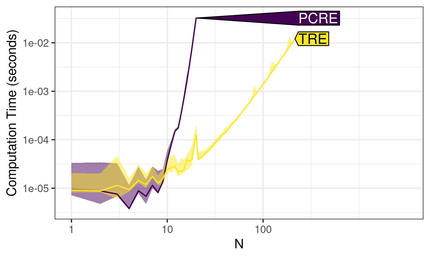

Figure 1: Comparing the computation time for using PCRE and TRE for regex matching with subjects and patterns of size N. Line shows the median, and the shaded band shows min/max, over 10 timings.

Note in the code above that the plot method returns a ggplot object, which we modify by adding null facets and a different y scale. By default, atime measures memory in kilobytes, as well as computation time in seconds. To simplify the discussion of this first example, we set the unit.col.vec element in the code above, which ensures that only the computation time is displayed (median line and min/max band over 10 timings). See Figure 4 for a more complicated example that also shows memory usage. Figure 1 shows the computation time for PCRE and TRE, making it easy to see the ranking of these libraries (TRE is faster than PCRE).

Asymptotic complexity class estimation

To estimate the asymptotic complexity class of each expression, we use the code below:

> (best.list <- atime::references_best(atime.list))

references_best list with 61 measurements, best fit complexity:
PCRE (2^N seconds)
TRE (N^3 seconds)

The code above fits an asymptotic reference curve for each of several complexity classes to each empirical timing curve. The complexity classes that are implemented by default include linear \(O(N)\), log \(O(\log N)\), quadratic \(O(N^2)\), exponential \(O(2^N)\), etc. The user can define complexity classes to use if the defaults are not sufficient. An asymptotic reference curve is fit for each complexity class by aligning it with the empirical curve for the largest \(N\) value. The output is the best fit asymptotic reference curve for each empirical curve, which is defined as the reference curve that is closest to the empirical curve, for the second to largest \(N\) value. To visualize the results, we use the code below.

> plot(best.list) + ggplot2::facet_grid(. ~ expr.name) +
+   ggplot2::scale_y_log10("Computation time (seconds)")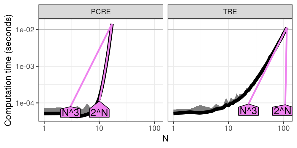

Figure 2: Computation time (seconds) as a function of input size N for PCRE and TRE. Empirical timings are shown in black (median line and min/max band over 10 timings), while violet curves show reference asymptotic growth rates: exponential O(2^N) is the best fit for PCRE, and cubic O(N³) is the best fit for TRE.

Figure 2 shows the timings of each expression as a function of data size \(N\) (black), as well as two asymptotic reference curves (violet, closest reference curve that is smaller/larger, with text labels that can be interpreted in terms of big O notation). Since we have chosen \(N\) and the time limit appropriately, we are able to observe the following. For small values of \(N\), the timings are dominated by the overhead, resulting in a nearly constant curve (especially for PCRE). As \(N\) increases, the PCRE curve becomes super-linear, indicating exponential complexity, as shown by the increasing slope in the log-log plot, and the almost perfect alignment between the black empirical curve and the violet exponential \(O(2^N)\) reference curve. Note that this example is a worst case for the PCRE library, which is actually quite fast for other, more typical subjects and patterns. The worst case is due to a pathological pattern and subject that induces catastrophic backtracking. For TRE, two references are shown: cubic \(O(N^3)\) appears to be the best fit, whereas exponential \(O(2^N)\) is the closest reference that is slower. Note that all polynomial references, including cubic \(O(N^3)\), appear as linear asymptotic trends on the log-log plot. Overall, Figure 2 shows the empirical timings, along with best fit asymptotic reference curves, which indicate that PCRE is exponential time, and TRE is polynomial time, as a function of the size of the subject/pattern \(N\).

Comparing latency and throughput

When comparing algorithms in terms of computational resources, we can either compare the time/memory required for a given data size \(N\) (latency), or show the data size \(N\) possible for a given time/memory budget (throughput). To compare latency for a given data size, we can simply subset the data table of empirical measurements, as below:

> atime.list$measurements[N==15, .(expr.name, seconds=median)]

   expr.name      seconds
1:      PCRE 0.0034745010
2:       TRE 0.0001235669

The output above shows that TRE is more than ten times faster than PCRE, at the given data size. To compare throughput, we use the code below.

> (pred.list <- predict(best.list))

atime_prediction object
      unit expr.name unit.value        N
1: seconds      PCRE       0.01  16.4573
2: seconds       TRE       0.01 109.7062

The output above shows a table with one row per expression. It shows that at the default time limit (0.01 seconds), TRE has a much larger estimated throughput than PCRE (N column). The throughput is estimated using linear interpolation on the log-log plot. The atime_prediction object has a plot method, which can be used to compare throughput, as in the code below.

> plot(pred.list) + ggplot2::facet_null() +
+   ggplot2::scale_y_log10("Computation time (seconds)", limits=c(NA, 5e-2))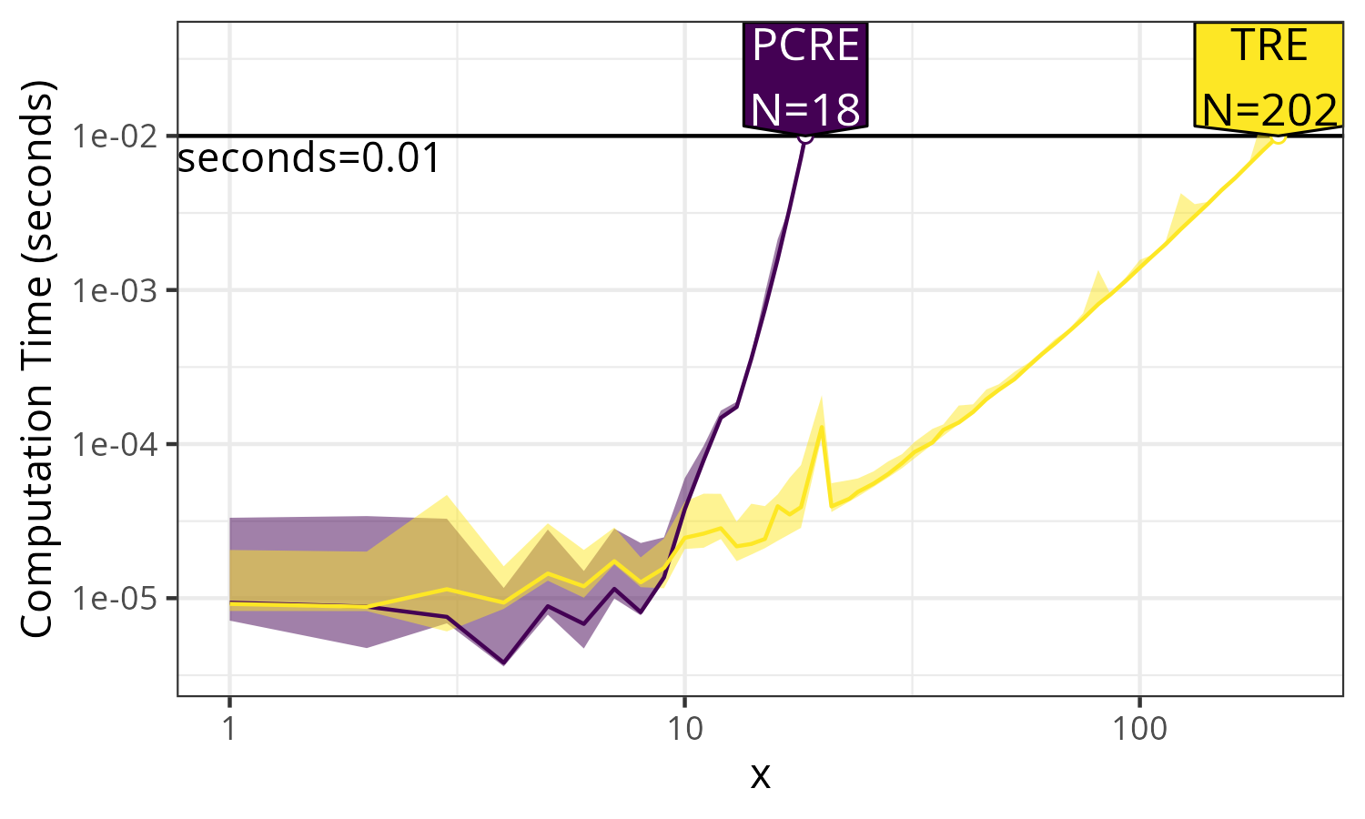

Figure 3: Computation time (seconds) versus data size (N= regex subject/pattern size), highlighting the largest data size N that can be processed within the default time limit of 0.01 seconds. Lines show median, and shaded bands show min/max, over 10 timings.

Figure 3 shows the throughput, which is the data size N that can be handled in a given amount of time. It is clear that the TRE can handle about 10x larger N for the given time limit.

4 Analyzing different units as a function of data size

In this section, we explain how atime can be used to analyze asymptotic properties of other units, in addition to computation time. We consider the example of creating vectors and matrices of size \(N\). In R, dense matrices are created using matrix(), whereas sparse matrices are created using Matrix(). The advantage of using a sparse matrix is that when the number of non-zeros is sub-quadratic, then the memory usage should also be sub-quadratic (whereas memory usage with a dense matrix would be quadratic). In the code below, we use atime to verify these properties, and we also compare with a one-dimensional numeric() vector (linear memory usage). Finally, the code below demonstrates usage of the result argument, which is a function applied to the result of each expression. Because this function returns a data frame with one row, the column in that data frame (length) is interpreted as another unit to analyze (in addition to default units, time in seconds and memory in kilobytes).

> library(Matrix)
> vec.mat.result <- atime::atime(
+   N = 10^seq(1, 7, by=0.25),  
+   vector = numeric(N),
+   matrix = matrix(0, N, N),
+   Matrix = Matrix(0, N, N),
+   result = function(x)data.frame(length = length(x)))
> plot(vec.mat.result)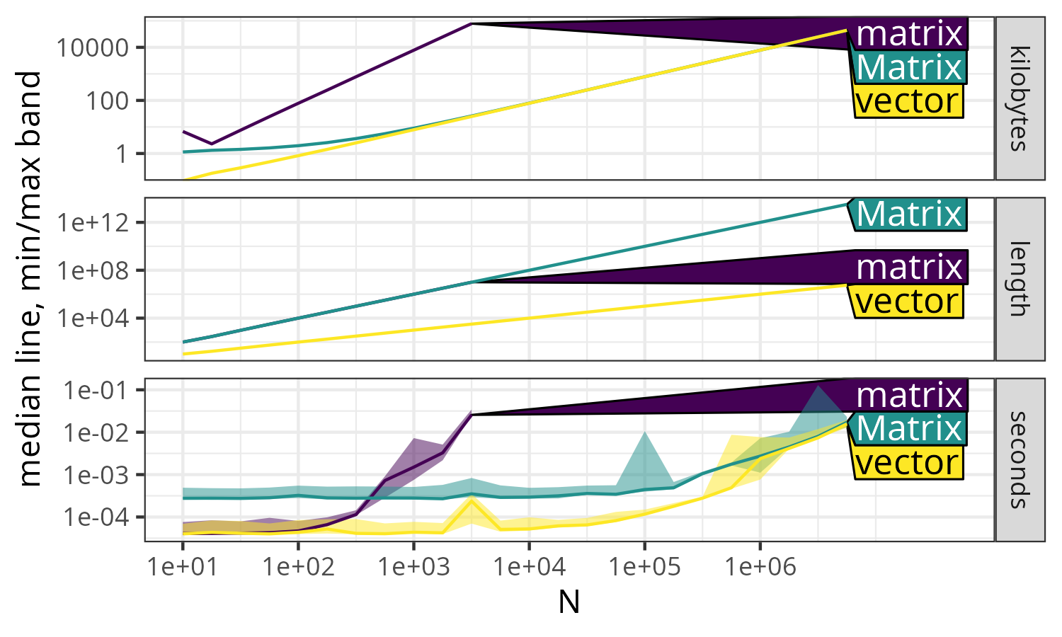

Figure 4: Asymptotic comparison of memory usage (kilobytes), object length, and execution time (seconds), for creating an N-vector, an N × N dense matrix, and an N × N sparse Matrix. The second panel shows median lines and min/max bands over 10 timings. Other panels show a line for the single measurement.

The code above creates Figure 4, in which there are three panels, each representing a different unit of measurement, as a function of data size \(N\).

Kilobytes:

This panel shows memory usage. The \(N\times N\) sparse Matrix and \(N\)-vector both exhibit linear \(O(N)\) asymptotic memory usage, while \(N\times N\) dense matrix requires quadratic \(O(N^2)\) memory, as shown by the greater slope in the log-log plot.

Length:

This panel represents the output of the length function. Both matrix and Matrix structures have the same quadratic \(O(N^2)\) length values, whereas vector has a smaller linear \(O(N)\) length asymptotically, as shown by its smaller slope on the log-log plot.

Seconds:

This panel displays execution time. For small values of N, Matrix is slower than both vector and matrix due to a small constant overhead. However, as N increases, Matrix and vector converge to the same linear \(O(N)\) asymptotic time complexity, much faster than the quadratic \(O(N^2)\) time matrix for large N.

As in the previous section, references_best() can be used to estimate asymptotic complexity classes, for each of the expressions (matrix, Matrix, vector), and each of the units (kilobytes, length, and seconds). Additionally, the predict() method can be used to estimate the throughput of each expression, for a given limit of seconds, kilobytes, and/or length.

Finally, we note that Figure 4 is a great example of the benefits of asymptotic measurement (as a function of N). In this example, we obtain different conclusions for different values of N:

N=10 to 100

Matrix is significantly slower than matrix, which is about the same as vector. But this observation is not indicative of performance in large data, because all methods are in the non-asymptotic regime (timings are dominated by constant overhead operations, which do not depend on the data). Also note the small spike for matrix at N=10, which may be attributed to garbage collection, and can be safely ignored since we are more concerned with performance for large N.

N=1,000 to 100,000

matrix is significantly slower than Matrix, which is significantly slower than vector. Again, this observation is not indicative of performance in large data, because Matrix and vector are in the non-asymptotic regime (but matrix is).

N=1,000,000 and more

matrix is significantly slower than Matrix, which is about the same as vector. This observation is indicative of performance in large data, because all methods are in the asymptotic regime (timings increase with data size).

The observations above highlight how the conclusions about which method is fastest depend on the data size N. Asymptotic analyses like Figure 4 are advantageous, because they allow the reader to immediately see if each method is in the asymptotic regime (which is desirable for comparing performance in large data).

5 Performance testing using atime

The atime package also provides functionality for performance testing R packages that are versioned using git. For performance testing an R package, we compute asymptotic time and memory usage for different git versions, and visualize the results to ensure that package code modifications do not result in performance regressions. In the context of our paper, a performance regression is a significant increase in execution time or memory usage for a particular test case. In this section, we explain how atime has been used to implement performance testing for data.table, an R package with users that depend on its impressive performance.

The atime package provides functions for prototyping test cases, defining test cases in an R package, and then running the test cases. The first step of performance testing is typically prototyping, which means experimenting with different test code, package versions, and data sizes until significant differences in performance can be observed. Prototyping is done using atime_versions(), which runs a given piece of R code, for several data sizes N, and for several package versions (defined using git SHA1 hashes). After prototyping, the arguments used with atime_versions() can be reused with atime_test(), which is used to define test cases in an R package. Finally, atime_pkg() can be used to run all test cases in an R package, or atime_pkg_test_info() can be used to extract test metadata and run one test at a time.

Prototyping performance tests using atime_versions()

The first step of performance testing is typically using atime_versions() for prototyping. Some arguments of atime_versions() are the same as atime(): N is a sequence of data sizes, and setup is an expression to create data for use in the test. The different package versions are specified as named arguments (Fast and Slow in the code below) whose values should be SHA1 hashes of the desired git versions. Additionally, pkg.path is the path to a local clone of a git repository containing the R package, and expr is an expression to time for each different package version. Note that this expression must contain a double or triple colon reference to the package name, such as data.table:::shallow() in the code below. This is necessary because the package name is replaced with an edited package name. Testing the different versions is implemented by installing different versions of the package to the same R package library. The different package versions have different names, so they can be loaded and run in the same R session. The names of the different R packages are created by appending the SHA1 hash to the package name, for example data.table.c4a2085e35689a108d67dacb2f8261e4964d7e12. The pkg.edit.fun argument is a function to edit the package, so that it can be installed and loaded using the versioned package name. A default pkg.edit.fun is provided that works with most R packages, including packages that use the Rcpp interface of Eddelbuettel and François (2011). The default editing function finds instances of the package name in source code and metadata files (such as DESCRIPTION, NAMESPACE, RcppExports.cpp), and replaces the package name with the edited package name. Because data.table has some special configuration and build files, it requires creating a custom function, edit.data.table(), see GitHub repository for details, https://github.com/Rdatatable/data.table/blob/master/.ci/atime/tests.R. We consider the example usage in the code below.

atime::atime_versions(
  pkg.path = "~/data.table",
  pkg.edit.fun = edit.data.table, 
  setup = {
    set.seed(1L)
    dt <- data.table(a = sample.int(N))
    setindexv(dt, "a")
  },
  expr = data.table:::shallow(dt),
  Slow = "b1b1832b0d2d4032b46477d9fe6efb15006664f4", 
  Fast = "9d3b9202fddb980345025a4f6ac451ed26a423be")

The code above runs a performance test on two different versions of the data.table package (Fast and Slow), involving computing a shallow copy of an indexed table with a variable number of rows \(N\). It is expected that this operation should be constant \(O(1)\) time, independent of the number of rows \(N\). When we use the plot method (Figure 5, left), we see that the Slow version time is increasing with \(N\), whereas the Fast version time is constant. Results like this, where significant differences can be observed between package versions, indicate that the code is a good candidate for a performance test. To summarize this section, atime provides the atime_versions() function, which can be used to compare the asymptotic performance of two git versions of an R package.

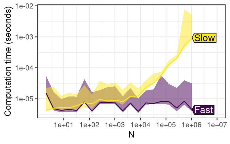
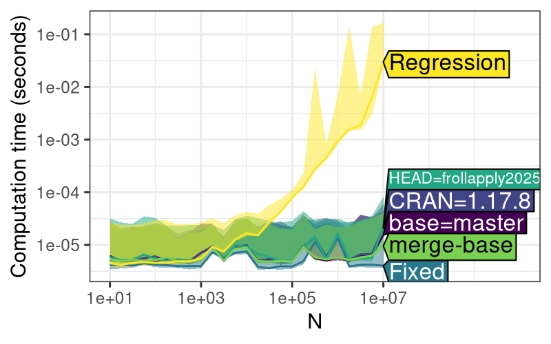
Figure 5: Left: plot() method for atime_versions() shows the asymptotic time taken for shallow(), which performs a shallow copy of a data table with N rows, an operation which is expected to be constant time (as in Fast version, but not Slow version). Right: the same test case ran in the context of a Pull Request on GitHub, resulting in three additional versions (CRAN, HEAD, base). It is clear that all versions other than Slow/Regression are about the same speed as Fast/Fixed, which indicates that HEAD is OK to merge into the base.

Defining performance tests in an R package

After having used atime_versions() to prototype a performance test, the next step is to move the test code into the R package. We propose defining performance test cases in the object named test.list defined in the pkg/.ci/atime/tests.R file, in a git repository pkg that contains an R package. Each element of the list should have an informative name for the test case, which will be used to display the results. Each value should be a list of named arguments to pass to atime_versions(), such as setup, expr, Fast, and Slow. Each test case is typically created based on a historical regression or performance improvement. For example, the R code below defines the test case involving shallow(), as discussed in the previous section.

test.list <- atime::atime_test_list(
  N = as.integer(10^seq(1, 7, by=0.25)),
  pkg.edit.fun = edit.data.table,
  "shallow speed improved in #4440" = atime::atime_test(
    setup = {
      set.seed(1L)
      dt <- data.table(a = sample.int(N))
      setindexv(dt, "a")
    },
    expr = data.table:::shallow(dt),
    Slow = "b1b1832b0d2d4032b46477d9fe6efb15006664f4", 
    Fast = "9d3b9202fddb980345025a4f6ac451ed26a423be"
  )
)

The code above uses the helper functions atime_test_list() and atime_test() to define the test case. Both functions are wrappers around list(), with non-standard evaluation for special arguments like setup and expr (un-evaluated expressions to pass to atime_versions). The arguments N and pkg.edit.fun are special names that are recognized by atime_test_list, and shared across all of the test cases in the list (only one test case shown above; see data.table repository for more). In addition to the code above, it is recommended to add names and/or comments that explain the origin of the test case. For example, the test case name "shallow speed improved in #4440" references the PR number, which resulted in the performance improvement. Also, for each SHA1 hash, we recommend a comment such as the following, which was used to document the origin of the Slow commit: Parent of the first commit (https://github.com/Rdatatable/data.table/commit/0f0e7127b880df8459b0ed064dc841acd22f5b73) in the PR (https://github.com/Rdatatable/data.table/pull/4440/commits) that improves speed. Such comments are useful because they can be used to double-check the validity of the SHA1 commit IDs. In this example, on the PR4440 web page, it can be seen that 0f0e712 is the first commit, and on that commit page, it can be seen that b1b1832 is indeed its parent (which is a good choice for a historical Slow reference because it occurred before the PR that introduced the performance improvement).

Running performance tests locally and on GitHub Actions

Running performance tests locally.

After having defined test cases as above, all the test cases in the package can be run locally by using atime_pkg("path/to/pkg"). It runs atime_versions() using the arguments provided in each test case, and then saves the results (RDS file), along with summary PNG figure files, to the directory pkg/.ci/atime. Alternatively, to run and visualize the results for a single test case, the code below can be used.

pkg.info <- atime::atime_pkg_test_info("~/R/data.table")
one.call <- pkg.info$test.call[["shallow regression fixed in #4440"]] 
one.result <- eval(one.call) 
plot(one.result)

The atime_pkg_test_info() function returns a list of information about the performance test cases, without actually running them yet. The pkg.info$test.call object is a list of un-evaluated expressions, each of which calls atime_versions() for a given test case. The code eval(one.call) runs one performance test, and the plot method can be used to visualize the results (Figure 5, right). Running the test case locally adds three versions (Table 2): HEAD (current git version in local clone), base (GITHUB_BASE_REF or master), and CRAN (current release). The performance of these versions can be compared to the historical commits (Fast and Slow) to evaluate the performance of the current code.

Running performance tests on GitHub Actions.

GitHub Actions is a continuous integration service that can run arbitrary code after every push to a git repository. A GitHub Action was created to facilitate performance testing of the changes that are introduced in a Pull Request (PR). The primary motivation behind this was to help ensure that data.table maintains its code efficiency as PRs are merged. The GitHub Action for performance testing can be enabled by creating a YAML file in pkg/.github/workflows (see atime web page for details). The GitHub Action first runs atime_pkg() after each push to a branch involved in a PR. The GitHub Action then creates a comment in the PR, with the summary figure that shows the result from the most recent performance test. The comment gets updated after each push to avoid cluttering the PR. The plot shows a column for each test case, with time and memory trends across different data.table versions (Table 2). In addition, the comment contains a link to download all the atime-generated result files (figure PNG files and RDS).

Several versions are provided automatically by atime, based on the context of the PR (base, HEAD, merge-base, CRAN). Other versions can be provided by the user based on what is relevant for each test case (Before, Regression, Fixed, Fast, Slow). For test cases that involve a regression, we recommend the version names Before, Regression, and Fixed, to indicate versions relative to the regression (Before and Fixed should be more efficient than Regression). For test cases that involve a performance improvement (or no known regression), we recommend using the version names Fast and Slow.

Table 2: Version names recognized by atime performance testing.

Version name	Defined?	Version description
Fast	user	An efficient commit
Slow	user	An inefficient commit
Before	user	An efficient commit before a performance regression
Regression	user	An inefficient commit affected by a performance regression
Fixed	user	An efficient commit after fixing a performance regression
CRAN	local	Latest version on CRAN
HEAD	local	Most recent commit in current branch
base	GitHub	Target branch of PR (typically main or master), if current branch is involved in a PR
merge-base	GitHub	The common ancestor between base and HEAD

6 Comparisons between textttatime and other software

Features of atime and touchstone for performance testing

In terms of performance testing functionality, the most similar R package to atime is touchstone, which also provides functions for performance testing, but without asymptotic measurement as a function of several data sizes.

Both touchstone and atime use relative performance testing, meaning that each test case is run using different versions of the R package. Touchstone allows specifying two branches, corresponding to the HEAD of a PR and its base branch. In addition to those branches, atime supports other branches that are important in the context of a PR (merge-base and CRAN), as well as user-defined commits that represent historical Fast/Slow versions.

touchstone::branch_install() installs each branch to a separate library, and uses callr to run each branch in a separate R process. In contrast, atime::atime_versions() installs each package version to the same library (using a different package name for each version). Therefore, atime allows the different R package versions to be loaded into the same R session, for more direct comparison (reduced noise).

Comparative benchmarking using atime::atime() and bench::press()

In terms of comparative benchmarking functionality, the function most similar to atime::atime() is bench::press(), which allows the user to specify several parameters to vary (not only data size N). The main advantage of atime is that it provides convenient features for benchmarking code that scales with data size, \(N\). For parameters other than N, the atime_grid() function can be used, as explained below.

Simple example with small data size \(N\), for which bench and atime work equally well.

The bench package can be used for asymptotic benchmarking, as long as the max data size \(N\) is chosen to yield a reasonable computation time for all expressions. For example, bench can be used to do a small-scale asymptotic comparison of PCRE and TRE, via the code below.

bench::press(
  N = 1:20,
  perl = c(TRUE, FALSE),
  with(create_subject_pattern(N), bench::mark(
    iterations = 10,
    regexpr(pattern, subject, perl = perl))))

The code above is an attempt to replicate Figure 1, but with smaller data sizes (max=20 instead of 1000, which would be too slow to compute using PCRE). In the code above, we use the bench::press() function to perform benchmarking across multiple parameter combinations (N and perl). For each combination, it uses create_subject_pattern(N) to generate a subject and pattern, and subsequently measures the performance of the regexpr function using bench::mark(). The regexpr function performs regular expression matching with the generated pattern on the subject, using the current value of perl to toggle Perl-compatible regex. The benchmarking process is repeated iterations = 10 times for each parameter combination. Below we show the analogous atime code.

atime::atime(
  N = 1:20,
  setup = N.data <- create_subject_pattern(N),
  expr.list = atime::atime_grid(
    list(perl = c(TRUE, FALSE)),
    regexpr = regexpr(N.data$pattern, N.data$subject, perl = perl)))

The code above uses the expr.list argument, which is a list of expressions to be benchmarked, constructed using atime::atime_grid, which defines a grid of parameter combinations, similar to bench::press(). In this case, the grid includes one parameter, perl, with values TRUE or FALSE. Overall, we see from this example that the atime and bench code is very similar, for the case where the max data size \(N\) is small enough to be computable by all expressions.

More complex example showing the advantage of atime.

An example that is more difficult to handle using bench::press() would be the analysis presented in Figure 4, which shows an extra unit (length, in addition to seconds and kilobytes), and involves very different time/memory scales (dense matrix is orders of magnitude less efficient than sparse Matrix). That analysis requires two useful features that are provided by atime().

• To measure quantities other than seconds and kilobytes as a function of N (such as length in Figure 4), a custom for loop is required with bench::press().

• If an expression takes longer than the time limit (default 0.01 seconds), then custom code is required for bench::press() to not be run for any larger N values. And in the case of Figure 4, it is also important to avoid running the large N values, to avoid running out of memory.

The 28 lines of code below can be used to achieve these two features using bench::press(), but it is complicated relative to the corresponding 6 lines of atime code that was used to create Figure 4 (see previous section).

seconds.limit <- 0.01
done.vec <- NULL
measure.vars <- c("seconds","kilobytes","length")
press_result <- bench::press(N = N_seq, {
  exprs <- function(...)as.list(match.call()[-1])
  elist <- exprs(
    vector=numeric(N),
    matrix=matrix(0, N, N),
    Matrix=Matrix(0, N, N))
  elist[names(done.vec)] <- NA #Don't run exprs which already exceeded limit.
  mark.args <- c(elist, list(iterations=10, check=FALSE))
  mark.result <- do.call(bench::mark, mark.args)
  desc.vec <- attr(mark.result$expression, "description")
  mark.result$description <- desc.vec
  mark.result$seconds <- as.numeric(mark.result$median)
  mark.result$kilobytes <- as.numeric(mark.result$mem_alloc/1024)
  mark.result$length <- NA
  for(desc.i in seq_along(desc.vec)){
    description <- desc.vec[[desc.i]]
    result <- eval(elist[[description]])
    mark.result$length[desc.i] <- length(result)
  }
  mark.result[desc.vec %in% names(done.vec), measure.vars] <- NA
  over.limit <- mark.result$seconds > seconds.limit
  over.desc <- desc.vec[is.finite(mark.result$seconds) & over.limit]
  done.vec[over.desc] <<- TRUE
  mark.result
})

The code above uses entries of done.vec to keep track of which expressions have already gone over the time limit. It also uses a for loop to evaluate each expression and save the length of the result to analyze as a function of N. Overall, the code is substantially more complex than the corresponding atime code, because it has to re-implement two features that atime provides.

To conclude this section, we have discussed the use of bench and atime packages for comparative benchmarking in R. Both methods can be used for comparative benchmarking across different parameter configurations. However, atime::atime() provides two key features which are not present in bench::press(): measurement of arbitrary units (other than time and memory), and stopping evaluation for expressions that go over a time limit.

Comparing overall time using different benchmarking packages

In this section, we provide an empirical comparison between atime and bench, in terms of how much time it takes overall to compute benchmark results. Our goal is to demonstrate an advantage of the proposed asymptotic approach implemented in atime: we can gather a larger range of measurements in a comparable or smaller amount of time.

First, we considered the regular expression example in Figure 1. The overall time taken by atime to compute the data for this benchmark was 1.7 seconds, and it resulted in a range of measurements (N=1 to 18 for PCRE, and N=1 to 151 for TRE). For comparison, we ran bench with various data sizes from N=19 to N=23, and we show the timings in Table 3. The most comparable amount of time for bench was 1.69 seconds for data size N=21, which is slightly larger than the largest data size for PCRE with atime (N=18), but significantly smaller than the largest data size for TRE with atime (N=151). Smaller data sizes were faster (0.42 seconds for N=19), and larger data sizes were slower (6.95 seconds for N=23).

Second, we considered the sparse matrix example in Figure 4. The overall time taken by atime to compute the data for this benchmark was 2.21 seconds, and it resulted in a range of measurements (N=10 to 3,000,000 for Matrix, N=10 to 3,000 for matrix, N=10 to 10,000,000 for vector). For comparison, we ran bench with various data sizes from N=5,000 to N=100,000, and we show the timings in Table 4. The most comparable amount of time for bench was 3.22 seconds for data size N=10,000, which is slightly larger than the largest data size for the matrix with atime (N=3,000), but significantly smaller than the largest data size for the other atime measurements (millions for Matrix and vector). Smaller data sizes were faster (0.66 seconds for N=5,000), and larger data sizes were either slower (11.53 seconds for N=20,000) or did not run (not enough memory to run the matrix for N=100,000).

Overall, the comparisons in this section have shown the advantages of the atime approach, which computes measurements for a range of data sizes until the median time exceeds a limit (default 0.01 seconds). The atime approach can be faster overall, for more informative results (measurements for a range of data sizes, not just one data size).

Table 3: Overall time required to compute regular expression benchmarks, as in Figure 1, using either bench (with various data sizes from 19 to 23) or atime (with the default time limit of 0.01 seconds, which results in a range of data sizes).

package	seconds	PCRE data sizes	TRE data sizes
bench	0.42	19	19
bench	0.81	20	20
bench	1.69	21	21
atime	1.70	1–18	1–151
bench	3.40	22	22
bench	6.95	23	23

Table 4: Overall time required to compute sparse/dense matrix benchmarks, as in Figure 4, using either bench (with various data sizes from 5000 to 100,000) or atime (with the default time limit of 0.01 seconds, which results in a range of data sizes).

package	seconds	Matrix data sizes	matrix data sizes	vector data sizes
bench	0.66	5000	5000	5000
atime	2.21	1e+01–3e+06	1e+01–3e+03	1e+01–1e+07
bench	3.22	10000	10000	10000
bench	11.53	20000	20000	20000
bench	out of memory	1e+05	1e+05	1e+05

Comparison with Python continuous benchmarking

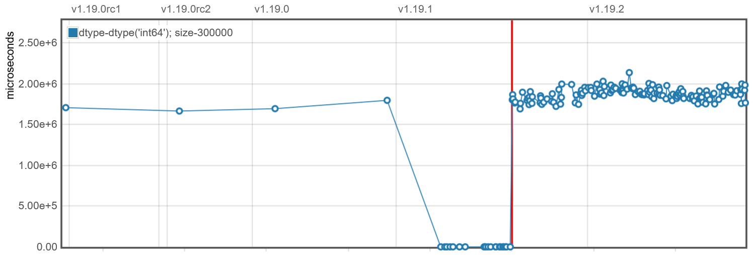
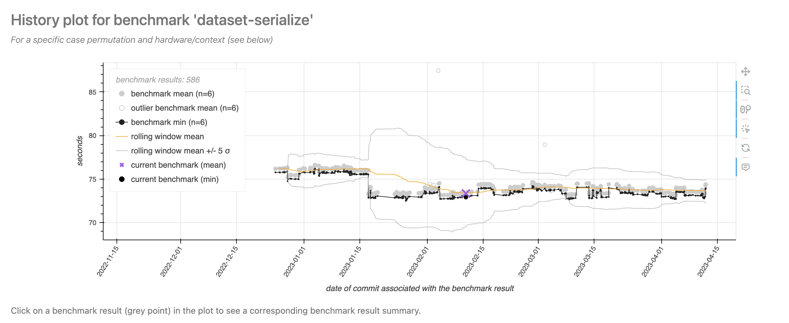
Python continuous benchmarking software includes airspeed velocity and conbench. Whereas the proposed atime method keeps a historical database of commits which are known to be Fast or Slow, these packages keep a historical database of timings for all commits (each timing computed once for that commit and then saved to compare with timings computed for other commits). Another major difference is that each atime test results in several measurements for a set of increasing data sizes, whereas these other tools use a fixed data size (which may not be relevant on different computer hardware). Assuming a relevant data size is used, these alternative approaches could be very useful, as performance regressions could be visualized as abrupt increases in computation time over the history of commits. Examples of web pages that are generated by these packages are shown in Figure 6, which show results taken from https://pv.github.io/numpy-bench/#bench_trim_zeros.TrimZeros.time_trim_zeros and https://conbench.github.io/conbench/pages/lookback_zscore.html. The limitation of this approach is that it requires careful control of the underlying hardware that was used to compute the benchmark timings for each commit. If there are variations in the hardware over time, that can result in false positive changes in benchmark computation time, which makes it more difficult to detect real performance regressions due to changes in the code. atime does not suffer from this drawback, because it computes timings for each data size and code version at test time on the same machine (Table 2), so it does not need to keep a database of historical benchmarks. Instead of presenting the user a time series plot with different code versions on the X axis, atime presents data size on the X axis (Figure 5), with different code versions represented as different colored empirical timing curves. False positives are, of course, still possible with atime, for example, because of “noisy neighbors” on shared virtual machines, or random garbage collection events, but these issues also affect other testing software.

Figure 6: Comparison with other continuous benchmarking software. Air Speed Velocity (top) and Conbench (bottom) are measurements of computation time for a fixed data size (Y axis), shown as a function of the commit history (X axis). The main drawback of this method is that it results in false positive changes up and down, as can be seen in these figures.

7 Discussion and conclusions

In this paper, we presented the atime package for comparative benchmarking of R code and performance testing in R packages. The unique feature of atime is asymptotic measurement of time and memory (as a function of data size), which makes it easy to see when the code performance is in the asymptotic regime (dependent on data size). The atime package enables users to compute and visualize asymptotic timings, including comparing empirical timings with theoretical references and estimating throughput. Several examples illustrated how atime can be applied for comparative benchmarking of different R functions that perform similar computations (but with different performance characteristics). Using data.table as an example, we explained how atime can be used for performance testing of R packages across multiple git versions.

Additionally, we compared atime’s syntax and functionality with other tools used for performance testing and benchmarking. Compared to other benchmarking tools (which support only a single data size), the unique feature of atime is support for sequences of data sizes. We showed that it is technically possible to use bench::press() for asymptotic analysis across a sequence of small data sizes, but atime is preferable because it supports convenience features such as stopping if a timing exceeds a time limit. Another similar package is touchstone, which provides a GitHub Action for performance testing based on comparing HEAD/base versions, but does not support asymptotic analysis (varying data sizes).

Limitations and future development.

A limitation of atime comes from the fact that it uses bench::mark() to measure time/memory for each data size. This dependency means that atime inherits both the strengths and limitations of bench::mark(). Because this method uses Rprofmem(), it is limited to measuring R memory allocations (and can not measure other C memory allocations). Also, this method runs timings for each expression several times, without re-running the setup expression. This makes it difficult to run timings on functions that alter their inputs by reference. For example, data.table::setkey(DT) alters DT by reference (sort in place); the first execution for memory measurement will sort the data, and subsequent executions for time measurement will do a linear scan to verify the data is sorted (faster). Future versions of atime could overcome this limitation by removing the dependency on bench and implementing a time/memory measurement procedure that runs the setup expression before each measurement.

Current use cases.

We note that atime is currently being used for continuous performance testing of data.table, with 16 test cases currently implemented, and running for every pull request on GitHub. The atime methodology has also been used to uncover and fix asymptotic performance issues in base R. For example, asymptotic analysis of write.csv() revealed that it was quadratic \(O(N^2)\) in the number of columns \(N\), whereas the expected complexity was linear \(O(N)\). Sebastian Meyer realized this issue was related to another issue with replacing columns via [.data.frame, which was observed to be super-linear, but expected to be linear. The fix for these two issues appeared in 2023 with R version 4.3.0. As mentioned in the introduction, atime has also been used for comparative benchmarking of CSV reading and writing functions (for details, see https://tdhock.github.io/blog/2023/dt-atime-figures/ and https://tdhock.github.io/blog/2024/pandas-dt/). Another improvement to base R was in substring(), which was expected to be linear \(O(N)\) time in the number of outputs \(N\), and gregexpr(), which was expected to be linear \(O(N)\) time in the number of characters \(N\) in the subject. Our asymptotic analysis revealed that both operations were quadratic \(O(N^2)\) time, and Tomas Kalibera merged the proposed fixes into R version 3.6.0 (2019). Overall, we have shown how atime simplifies such asymptotic analysis, and we expect that it will be a useful tool for future analyses of other R functions.

Reproducible research statement: The following repositories contain all the code for reproducing the figures in this paper:

https://github.com/tdhock/atime-article
https://doi.org/10.5281/zenodo.14796684

8 CRAN packages used

data.table, microbenchmark, bench, atime, rbenchmark, testComplexity, airspeed velocity, conbench, bencher, pytest-benchmark, pytest, touchstone, Rcpp, callr

9 CRAN Task Views implied by cited packages

ChemPhys, Finance, HighPerformanceComputing, NumericalMathematics, TimeSeries, WebTechnologies

10 Note

This article is converted from a Legacy LaTeX article using the texor package. The pdf version is the official version. To report a problem with the html, refer to CONTRIBUTE on the R Journal homepage.