1 Introduction
The Neyman-Scott point process (Neyman and Scott, 1958) is a cluster point process model widely used in biology, astronomy, forestry, medicine, etc. Its main advantages are the straightforward interpretation of the model parameters and the closed form of moment properties, at least for the stationary version of the model.
The model can be constructed in two stages and it is often called a doubly stochastic process: first, cluster centers are randomly sampled from a given Poisson point process; second, conditionally on the positions of cluster centers, a random number of offspring points are randomly and independently placed around each cluster center. Thus, the stationary Neyman-Scott point process model is specified by the intensity of the Poisson process of cluster centers, the distribution of the number of points per cluster (hereafter called cluster size), and the distribution of the relative displacement of the offspring points around their respective cluster centers (hereafter called cluster spread).
In the most popular type of Neyman-Scott point process, called the (modified) Thomas process (Thomas, 1949), the cluster size is assumed to follow a Poisson distribution and the cluster spread is governed by a radially symmetric Gaussian distribution. The stationary Thomas process is then described by the following parameters: the intensity \(\kappa\) of the process of cluster centers, the mean number of points in a cluster \(\alpha\) and the standard deviation \(\omega\) of the Gaussian distribution determining cluster spread.
A natural way of introducing inhomogeneity into the Neyman-Scott process model is allowing some of the model components (intensity of cluster centers \(\kappa\), cluster size \(\alpha\), cluster spread \(\omega\)) to depend on a set of spatial covariates. Their significance then needs to be assessed. Several models of this type have been studied in the literature, as discussed in the following paragraphs.
The Neyman-Scott point process with inhomogeneous cluster centers, with the distribution of the clusters being the same in terms of size and spread, allows for varying the number of clusters in the space. The inference for this process was investigated in Mrkvička et al. (2014) and it was found that the Bayesian MCMC estimation procedure is more precise than composite likelihood or minimum contrast method. This model is not second-order inhomogeneity reweighted stationary (SOIRS) (Baddeley et al., 2000), but if instead the mean number of points in a cluster \(\alpha\) is inhomogeneous, the resulting process is very close to SOIRS. The inference for SOIRS Neyman-Scott process (stationary Neyman-Scott point process thinned by a spatially varying function) can be performed by a two step method based on minimum contrast or composite likelihood (Waagepetersen and Guan, 2009), as implemented in the R package spatstat (Baddeley et al., 2015).
The inhomogeneity can be also introduced in the cluster spread \(\omega\), then the process will be locally-scaled Neyman-Scott point process (Hahn et al., 2003). It is also possible to introduce inhomogeneity simultaneously in \(\alpha\) and \(\omega\), then the process can be called a Neyman-Scott point process with growing clusters (Mrkvička, 2014).
For the models with homogeneous population of cluster centers but inhomogeneity in the cluster properties we talk about cluster inhomogeneity. On the other hand, for the Neyman-Scott point process with inhomogeneous cluster centers we talk about inhomogeneity of centers. Combining the cluster inhomogeneity and inhomogeneity of centers leads to the notion of doubly inhomogeneous Neyman-Scott point process. The Bayesian MCMC inference for such a process was studied in (Mrkvička and Soubeyrand, 2017). Other kinds of inference were found to be useless for such a complex model.
Therefore, we build up the R package binspp which contains the Bayesian MCMC estimation procedure for the most general model with inhomogeneity in all three model components. This model contains all the previous models as special cases, including the stationary one. The radially symmetric Gaussian distribution is assumed to determine the cluster spread, which does not limit practical applicability of the models. We do not include SOIRS Neyman-Scott point process due to the different construction of the model and also due to availability of moment-based estimation methods. However, practically speaking the Neyman-Scott point process with inhomogeneous cluster size \(\alpha\) can be used as an approximation to the SOIRS Neyman-Scott point process model.
The most important statistical problem here is to assess the dependence of the data on the given set of covariates. Our package handles the spatial covariates influencing any or all of the model components: the intensity of the cluster centers \(\kappa\), the cluster size \(\alpha\) and the cluster spread \(\omega\). The Bayesian MCMC procedure is time consuming, but its great benefit is that the significance of all covariates is provided from the estimated posterior distributions in a natural way. For example, in case of the inhomogeneity of cluster centers if a faster estimation method is used, it is necessary to perform parametric bootstrap in order to obtain the significance of the covariates. This is as time consuming as the Bayesian MCMC procedure (Mrkvička et al. 2014). Only in the case of SOIRS Neyman-Scott processes it is possible to use the fast estimation method and the significance of covariates can be assessed using the asymptotic normality result obtained in Waagepetersen and Guan (2009).
As mentioned above, the minimum contrast approach and the composite likelihood approach are available for SOIRS Neyman-Scott point process. They are also described in Mrkvička et al. (2014) for the Neyman-Scott point process with inhomogeneous cluster centers. To the best of our knowledge, they are not available for the other kinds of inhomogeneity discussed above.
In order to model inhomogeneous clustered point patterns log-Gaussian Cox process (LGCP) models are often used (Møller et al., 1998). The inference for SOIRS LGCP is well developed with integrated nested Laplace approximation (INLA) (Rue et al. 2009) available through the package inlabru (Bachl and Lindgren 2020), with Bayesian MCMC inference available through the package lgcp (Taylor et al. 2020) or with the moment methods available through the package spatstat. Nevertheless, none of these packages allows for inference for LGCP with more complex types of inhomogeneity. An attempt in this direction has been made in (Dvořák et al., 2019).
With these considerations in mind, we have implemented the core functions of the binspp package using Rcpp to speed up the computation. As a result, short runs of the chain, useful for tuning up the hyperparameters of the prior distributions, are finished within minutes on a regular laptop. Long runs, used for the actual estimation, may be finished within a few hours, see the detailed example in Section 4.5. This makes our implementation easily applicable in practice, without the need to worry about the computational demands.
The inference for Neyman-Scott point processes is usually performed with the assumption of Poisson distribution of the number of points in a cluster. The same is assumed in all models discussed above, but the binspp package contains also the Bayesian MCMC estimation procedure for homogeneous generalised Neyman-Scott process. The method was described in (Andersson and Mrkvička, 2020). This model uses the generalised Poisson distribution (GPD) as a distribution of the number of points in a cluster. The GPD allows for modelling of under- or over-dispersion. This allows for more flexible modelling of the distribution of the number of points in a cluster.
The package specifically considers the following models. The inhomogeneous Thomas point process allowing for modelling of cluster centers, cluster spread and cluster sizes through covariates. The covariates are incorporated in every model component via exponential model. Such a general process was not presented in the literature, even (Mrkvička and Soubeyrand, 2017) presents only a special case of this general model. Furthermore, the generalised Neyman-Scott point process which allows for modelling underdispersed or overdispersed cluster sizes is considered.
This paper is organized as follows. First, in Section 2 we describe the models considered here. Then we briefly describe the algorithms in Section 3. In Section 4 we show the use of our package for different types of models, with a detailed example in Section 4.5 considering a real dataset of infected oak trees. This is a part of a larger dataset studied in Fernández-Habas et al. (2019). The model for the observed point pattern includes inhomogeneity in all three components of the model and for illustration we provide the outputs of a long run of the MCMC chain. We also show in Section 4.7 the use of the estimation procedure for homogeneous generalised Neyman-Scott point process and the possibility of detecting over- or under-dispersion of cluster sizes. Section 5 is left for discussion.
2 Models
Let us first describe the model in its full generality, i.e. the doubly inhomogeneous Neyman-Scott point process. The process of cluster centers \(C\) follows an inhomogeneous Poisson point process with intensity function \(\kappa f (\beta, u), \ u\in W \subset \mathbb{R}^2\), where \(\kappa > 0\) and \(\beta \in \mathbb{R}^k\) are parameters. The clusters \(X_c, c \in C\), are independently attached to every cluster center \(c\). The Neyman-Scott point process is the superposition of the clusters \(X=\cup_{c\in C} X_c\), where \(X_c\) are independent Poisson point processes with intensity function \(\alpha (\mu,c)k(u-c, \omega (\nu,c)), u \in \mathbb{R}^2\), which depends on \(c\). Here \(\alpha(\mu, c)\) is the expected number of offspring points in the cluster corresponding to the parent point \(c\) and \(\mu \in \mathbb{R}^{l+1}\) is a parameter. Furthermore, \(k(\cdot, \omega(\nu, c))\) is the probability density function governing the relative displacement of the offspring points around the parent point \(c\) (in this paper we assume \(k\) is the density of the centered radially symmetric normal distribution with the standard deviation \(\omega(\nu, c\))). The distribution of the number of points in the cluster with the cluster center \(c\) is assumed to be Poisson for all inhomogeneous models, with the probabilities being denoted \(p(n, \alpha(\mu, c))\).
The parametric functions \(f\), \(\alpha\) and \(\omega\) are the key ingredients of the model which describe the dependence on the spatial covariates. These functions are assumed to take the following parametric form: \[\begin{align*} f(\beta,u) & = \exp(\beta_1 z_1(u)+\ldots + \beta_k z_k(u)), \\ \alpha(\mu,c) & = \exp(\beta^\alpha_0+\beta^\alpha_1 z^\alpha_1(c)+\ldots + \beta^\alpha_l z^\alpha_l(c)), \\ \omega(\nu,c) & = \exp(\beta^\omega_0+\beta^\omega_1 z^\omega_1(c)+\ldots + \beta^\omega_m z^\omega_m(c)). \end{align*}\]
Here \(z_1, \ldots , z_k\) are the spatial covariates influencing the population of cluster centers, \(z_1^\alpha, \ldots , z_l^\alpha\) are the spatial covariates influencing the cluster size and \(z_1^\omega, \ldots , z_m^\omega\) are the spatial covariates influencing the cluster spread. All the \(\beta\)s are real-valued regression parameters. Note that the model for \(f\) does not contain the intercept since its role is taken by the parameter \(\kappa\). We use this parametrization to be consistent with the earlier works describing the models and the corresponding Bayesian inference (Mrkvička, 2014; Kopecký and Mrkvička, 2016; Mrkvička and Soubeyrand, 2017).
Specific choices of \(k,l,m\) result in different special cases of the general model. For \(k = 0, l = 0, m = 0\) the process is the stationary Neyman-Scott process. For \(k > 0, l = 0, m = 0\) we obtain the inhomogeneous cluster centers. Similarly, \(k = 0, l > 0, m = 0\) results in inhomogeneous cluster sizes, while \(k = 0, l = 0, m > 0\) leads to locally scaled process (inhomogeneous cluster spread). For \(k = 0, l > 0, m > 0\) we obtain the process with growing clusters (Mrkvička 2014) and finally for \(k > 0, l > 0, m > 0\) we obtain the most general, doubly inhomogeneous process (Mrkvička and Soubeyrand, 2017).
Our package allows for all the possible choices of \(k, l, m\). However, the user must be aware of the possible identifiability issues which occur if the same covariate is used for \(z_i\) and \(z_j^\alpha\) for some \(i\) and \(j\), i.e. if the same covariate influences both \(f\) and \(\alpha\). It is a property of the two-step estimation algorithm described in the next section that the parameters \(\beta_i\) and \(\beta_j^\alpha\) cannot be estimated correctly in this case. For example, if \(\beta_i = 0\) and \(\beta_j^\alpha \neq 0\) then the first step of the algorithm will estimate \(\hat\beta_i\) to be approximately \(\beta_j^\alpha\).
The binspp package allows also for the estimation of the homogeneous generalised Neyman-Scott point process, where the distribution of the cluster sizes follows the generalised Poisson distribution, which is a popular model for count data (Wang and Famoye, 1997). The probability mass function of GPD is \[\begin{align*} p(n|\lambda, \theta) = \left\{\begin{array}{l} \frac{1}{n!}\theta(\theta + \lambda n)^{n-1}e^{-\theta-\lambda n}, \quad n = 0, 1, 2, \ldots, \\ 0, \quad \quad \text{if } n > \tilde n \text{ when } \lambda <0, \end{array} \right. \end{align*}\] where \(\theta > 0\), \(| \lambda | < 1\), and \(\tilde n\) is the largest integer such that \(\theta + \lambda \tilde n > 0\) when \(\lambda < 0\). When \(\lambda < 0, p(n|\lambda, \theta)\) does not sum to 1, and needs to be renormalized. The expectation is equal to \(\alpha = \frac{\theta}{1-\lambda}\), and variance is equal to \(\frac{\theta}{(1-\lambda)^3}. \label{eq:V}\) The parameter \(\lambda \in [-1,1]\) in GPD models the over- or under-dispersion, \(\lambda=0\) corresponds to the Poisson case, \(\lambda>0\) to the over-dispersed and \(\lambda<0\) to the under-dispersed case.
3 Inference
The inference for the doubly inhomogeneous Neyman-Scott point process observed in a bounded observation window W is performed in two steps, similar to the approach of (Waagepetersen and Guan, 2009).
In the first step, the parameters \(\overline{\beta}=(\log (\lambda) ,\beta_1, \ldots, \beta_k)\) of the intensity function are estimated, based on the assumption that \(X\) is the Poisson process with the intensity function \[\begin{align} \label{aprox} \overline{f}_{\overline{\beta}} (u) = \exp (\overline z(u) \overline \beta^T), \ u \in \mathbb R^2, \end{align} \tag{1}\] where \(\overline z(u) = (1, z_1(u), \ldots , z_k(u))\). This assumption is intuitively justified if the range of interaction among the points is small compared to the range of changes in the spatial covariates and if \(z_i\) is different from \(z_j^\alpha\) for all combinations of \(i\) and \(j\). Specifically, we maximize the log-likelihood of the assumed inhomogeneous Poisson process: \[\begin{align} l(\overline{\beta})=\sum_{x\in X \cap W} \overline z(x)\overline{\beta}^T - \int_W \exp (\overline z(u)\overline{\beta}^T) \, \mathrm{d}u \end{align}\] Here \(W\) is the observation window.
The second step consists of estimation of the interaction parameters \(\mu\) and \(\nu\), conditionally on the estimate of \(\overline{\beta}\).
Bayesian estimation for the homogeneous Neyman-Scott point processes was carried out with an MCMC algorithm e.g. in (Guttorp and Thorarinsdottir, 2012; Møller and Waagepetersen, 2007; Mrkvička, 2014; Kopecký and Mrkvička, 2016). In this approach, the cluster centers and the model parameters are updated in each step of the MCMC algorithm. After reaching the equilibrium, posterior distributions of the parameters can be estimated. The cluster centers are generally viewed as nuisance parameters.
Considering the inhomogeneous clusters, the MCMC algorithm proceeds in the same way as in the homogeneous case, except that the likelihood is influenced by the parameters connected with the cluster inhomogeneity. We remark here that the estimation algorithm was not presented in such generality earlier, even (Mrkvička and Soubeyrand, 2017) considered only a special case of this model, without allowing for the general form with covariates. However, the generalisation is straightforward.
Let \(C\) denote the inhomogeneous Poisson point process of cluster centers with the intensity \(\kappa f(\beta, u)\). Let \(p(C|\kappa, \beta)\) denote the Poisson probability density function of the point process \(C\), conditionally on \(\kappa\) and \(\beta\), with respect to the distribution of the unit-rate homogeneous Poisson point process. Furthermore, let \(p(X|C, \beta, \kappa, \mu, \nu)\) denote the Poisson probability density function of the point process \(X\) under the knowledge of \(C\), \(\beta\), \(\kappa\), \(\mu\) and \(\nu\). The joint posterior distribution of the process \(C\) and the parameters is then \[\begin{align} p(C, \kappa, \mu, \nu |X) \propto p(X|C, \beta, \kappa, \mu, \nu) p(C|\kappa, \beta) p(\mu) p(\nu), \end{align}\] where \(p(\mu)\) and \(p(\nu)\) denote the prior probability density functions for the respective parameters. No prior for \(\kappa\) is required because it is, in our estimation procedure including a modification similar to the one proposed by Kopecký and Mrkvička (2016), a deterministic function of \(\mu\) and \(\beta\). Indeed, the expected number \(\mathbb E M\) of the observed points in the observation window \(W\) is equal to \[\begin{align*} \kappa \int_W \alpha(\mu, u) \left[\int_{\mathbb R^2} k(u-c,\omega (\nu, c))f(\beta, c) \, \mathrm{d}c \right] \, \mathrm{d}u, \end{align*}\] which can be approximated by \[\begin{align*} \mathbb E M \approx \kappa \int_W \alpha(\mu, u))f(\beta, u) \, \mathrm{d}u. \end{align*}\] Thus, in each iteration of the MCMC algorithm, \(\kappa\) can be re-computed when \(\mu\) is updated.
Our MCMC algorithm consists of updating the process of cluster centers \(C\) and updating the parameters \(\mu\) and \(\nu\). For updating \(C\) we use the birth-death-move algorithm described in Møller and Waagepetersen (2004). For updating \(\mu\) and \(\nu\) we use the Metropolis-Hastings algorithm. In order to obtain better mixing properties \(\mu\) and \(\nu\) are updated separately. Full details about this algorithm can be found in (Mrkvička and Soubeyrand, 2017).
The inference for the interaction parameters \(\mu\) and \(\nu\) is performed from the estimated posterior distributions which are obtained from the MCMC samples after appropriate burn-in. The inference about the first-order inhomogeneity parameters \(\beta\) cannot be obtained from the first step where the Poisson distribution is assumed. Therefore, we base the inference about \(\beta\) on the posterior distribution of the cluster centers obtained in the second step. In every step the significance of \(z_1, \ldots, z_k\) with respect to the process of cluster centers \(C\) is assessed using the Poisson distribution of \(C\) assumed in this model. The median of respective \(p\)-values computed from the posterior distribution is taken to be the estimate of the \(p\)-value of the test of significance of the given covariate. We remark that it is also possible to perform the full Bayesian estimation by considering the inhomogeneity of cluster centers in the MCMC procedure. However, this approach was found to be less efficient than the two-step approach due to identifiability issues in the full likelihood.
Considering the generalised Neyman-Scott process, the MCMC algorithm consists of one extra step in addition to the traditional Metropolis-Hastings update of the model parameters and the birth-death-move update of the cluster centers. It is the update of the connections between the points and the cluster centers, since by assuming the non-Poisson distribution these connections take part in the likelihood of the process. Full details about this algorithm can be found in (Andersson and Mrkvička, 2020).
4 Examples
In this section we provide a set of examples illustrating how different types of models can be fitted using the Bayesian MCMC approach implemented in the binspp package. The first few examples illustrate the use of the package, while the most complex example in Section 4.5 describes the outputs of the algorithm in full detail. Model parametrization is described in Section 2.
Below we assume that X is the observed point pattern in the ppp
format used in the spatstat package. We further assume that X is
observed through the observation window W, which is a union of aligned
rectangles, aligned with the coordinate axes. x_left, x_right,
y_bottom and y_top are vectors giving the coordinates of the
extreme points of the rectangles whose union forms the observation
window W.When the observation window is rectangular, it is possible to
supply it using the argument W in the estimation function instead of
the vectors x_left to y_top. Furthermore, W_dil is the dilated
observation window used to accommodate cluster centers outside W to
mitigate the edge effects. An easy way to obtain W_dil from the
vectors x_left to y_top is shown in Section
4.5. All covariates such as cov1 are
assumed to be pixel images (objects of type im from the spatstat
package) defined over the W_dil domain.
The list control contains important tuning constants such as the
required number of iterations to be run (NStep), the length of the
initial part of the chain to be discarded before computing estimates
(BurnIn) or the sampling frequency used to reduce autocorrelations in
the values used for computing the estimates (SamplingFreq). Also,
hyperparameters for prior distributions for different parameters can be
specified in this list, as illustrated in the detailed example in
Section 4.5. Providing hyperparameter values
guided by the knowledge of the problem at hand is highly recommended!
However, some default values are used if the user does not provide them.
All priors are normal distributions, priors for \(\beta_i^\alpha\) and \(\beta_i^\omega\), \(i>0\), have expectation 0. We remark here that also the hyperparameters for \(\beta_0^\alpha\) and \(\beta_0^\omega\) must be given in \(\log\) scale because all parameters, except \(\kappa\), are estimated in the exponential form.
The estimation algorithm runs an MCMC chain of all the model parameters
(and the process of cluster centers). The chain converges to the
equilibrium state corresponding to the posterior distribution. The
values of the MCMC chain can be accessed using the rawMCMCoutput
function, providing samples from the posterior distribution of the model
parameters. The tuning constants given in the control argument specify
how the MCMC algorithm is run. NStep gives the required number of
steps of the chain, and BurnIn gives the number of initial steps to be
disregarded so that the equilibrium state is reached. The equilibrium
state can be determined by various diagnostic plots provided by the
package. E.g. the log-likelihood does not increase anymore, the number
of centers is stabilized, the trace plots of the parameters show
stationary behavior, and the histograms of posterior distributions are
unimodal. The value SamplingFreq controls how many steps of the chain
are made before recording a new sample. This helps control the
dependence between the sampled values. The bigger the SamplingFreq,
the lower the correlation, but fewer samples are obtained.
Homogeneous Thomas process
First, we simulate a point pattern using the spatstat function
rThomas and specify the observation window. In the following examples,
we do not explicitly include these commands for conciseness.
library(spatstat)
library(binspp)
W     <- square(1)
W_dil <- dilation.owin(W,0.1)
X     <- rThomas(30, 0.02, 5, W)
Then we set up the control parameters. Based on our experience, for this homogeneous model we recommend running at least \(50\,000\) iterations, with burn-in of at least \(25\,000\) steps.
control <- list(NStep=50000, BurnIn=25000, SamplingFreq=10)The following commands provide equivalent ways of specifying that all three components of the model are homogeneous (no covariates are provided):
Output <- estintp(X=X, control=control, W=W, W_dil=W_dil)
Output <- estintp(X=X, control=control, W=W, W_dil=W_dil,
                  z_beta=NULL, z_alpha=NULL, z_omega=NULL)
Output <- estintp(X=X, control=control, W=W, W_dil=W_dil,
                  z_beta=list(), z_alpha=list(), z_omega=list())
In this example the default hyperparameter values were used. These can be retrieved in the following way:
Output$priorParametersThe text outputs and graphical outputs are obtained as follows:
print(Output)
plot(Output)
Thomas process with inhomogeneous cluster centers
In this example the population of parent points is inhomogeneous, with
intensity function depending on a covariate. More covariates can be
included in the model, provided they are given in the z_beta list,
see Section 4.5 for an illustration.
For this model with simple inhomogeneity we recommend running at least
\(100\,000\) iterations, with burn-in of at least \(50\,000\) steps. Note
that the covariates in the list z_beta must be named in order for the
ppm function from the spatstat package to run properly. We first
create a simple covariate describing the \(x\)-coordinate.
cov1    <- as.im(function(x,y){x}, W=W_dil)
control <- list(NStep=100000, BurnIn=50000, SamplingFreq=10)
Output  <- estintp(X=X, control=control, W=W, W_dil=W_dil,
                  z_beta=list(Z1=cov1))
Thomas process with inhomogeneous mean number of points in a cluster
Now we assume that the mean number of points in a cluster depends on the
position of the corresponding parent point \(c\), with the function
\(\alpha(\mu,c)\) depending on a covariate. Again, more than one covariate
may be used, provided they are given in the z_alpha list.
For this model with simple inhomogeneity we recommend running at least \(100\,000\) iterations, with burn-in of at least \(50\,000\) steps.
control <- list(NStep=100000, BurnIn=50000, SamplingFreq=10)
Output  <- estintp(X=X, control=control, W=W, W_dil=W_dil,
                  z_alpha=list(cov1))
Thomas process with inhomogeneous cluster spread
In this case the spread of the clusters depends on the position of the
corresponding parent point \(c\), with the function \(\omega(\nu,c)\)
depending on a covariate. As before, more than one covariate may be
given in the z_omega list.
For this model with simple inhomogeneity we recommend running at least \(100\,000\) iterations, with burn-in of at least \(50\,000\) steps.
control <- list(NStep=100000, BurnIn=50000, SamplingFreq=10)
Output  <- estintp(X=X, control=control, W=W, W_dil=W_dil,
                  z_omega=list(cov1))
Thomas process with complex inhomogeneities in all model components
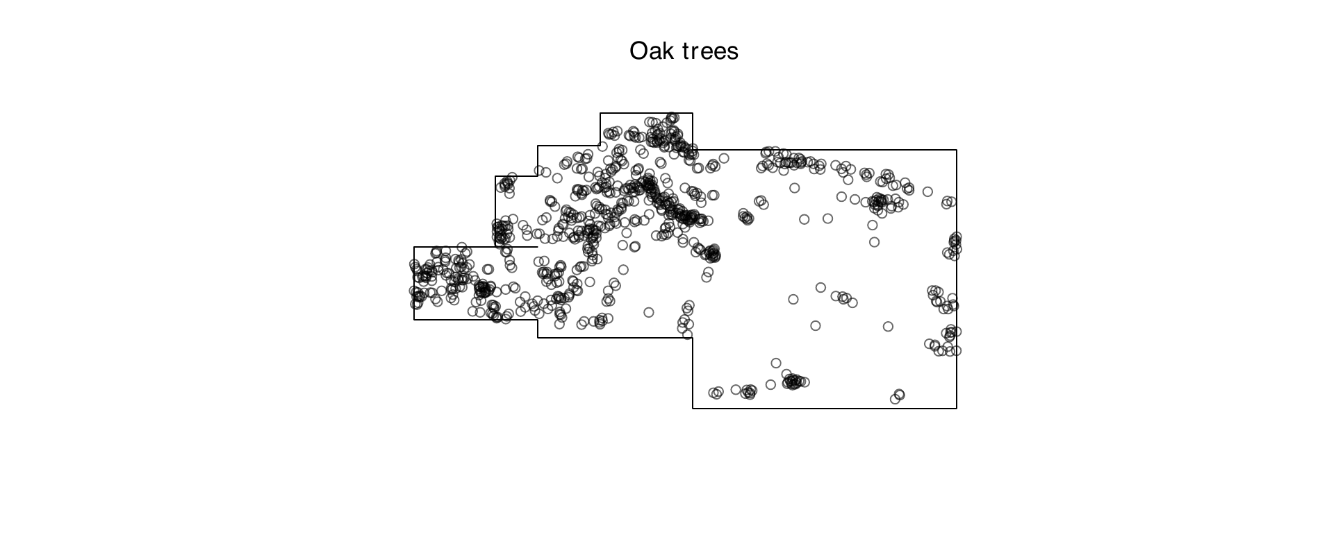
For this example we use the real dataset provided in the binspp
package, see also (Fernández-Habas et al. 2019).The dataset is shown in
Figure 1 and it
can be plotted using plot command as usual. The aim of this example is
to show the possibility of modeling simultaneously the inhomogeneous
centers of clusters, inhomogeneous cluster sizes and inhomogeneous
cluster spread, using the lists of covariates z_beta, z_alpha and
z_omega. The presented methodology is the only available methodology
that allows for such a complexity.
X        <- trees_N4
x_left   <- x_left_N4
x_right  <- x_right_N4
y_bottom <- y_bottom_N4
y_top    <- y_top_N4
Several covariates accompany the observed point pattern. In the
following lists we specify which covariates are assumed to influence
which model components. Note that each model component depends on two
covariates. Due to identifiability reasons the lists z_beta and
z_alpha must be disjoint (no covariate can appear in both lists).
z_beta  <- list(refor=cov_refor, slope=cov_slope)
z_alpha <- list(tmi=cov_tmi, td=cov_tdensity)
z_omega <- list(slope=cov_slope, reserv=cov_reserv)
The observation window is given as the union of aligned rectangles, aligned with the coordinate axes.
W <- owin(c(x_left[1],x_right[1]),c(y_bottom[1],y_top[1]))
if(length(x_left)>=2){
  for(i in 2:length(x_left)){
    W2 <- owin(c(x_left[i],x_right[i]),c(y_bottom[i],y_top[i]))
    W <- union.owin(W,W2)
  }
}
The dilated observation window is obtained as follows:
W_dil <- dilation.owin(W,100)The parameter 100 for the dilation specifies the width of the zone
around W where centers having offsprings in W can occur. Since the
Gaussian distribution for the offsprings is used, the width is infinite
in theory, but for computational reasons we bound this region.
For this model with complex inhomogeneities we recommend running at least \(250\,000\) iterations, with burn-in of at least \(150\,000\) steps. Hyperparameter values for prior distributions can be specified as follows:
control <- list(NStep=250000, BurnIn=150000, SamplingFreq=10, Prior_alpha_mean=3,
              Prior_alpha_SD=2, Prior_omega_mean=5.5, Prior_omega_SD=5,
              Prior_alphavec_SD=c(4.25,0.012), Prior_omegavec_SD=c(0.18,0.009))
The following commands perform the MCMC estimation. With the required 250 000 steps of the algorithm the computation takes approx. 2.5 hours on a regular laptop due to the implementation of the core functions using the Rcpp package.
set.seed(12345)
Output <- estintp(X=X, control=control, x_left=x_left, x_right=x_right,
                  y_bottom=y_bottom, y_top=y_top, W_dil=W_dil,
                  z_beta=z_beta, z_alpha=z_alpha, z_omega=z_omega)
Text output, providing the parameter estimates (medians of the estimated posterior distributions) together with the corresponding 2.5% and 97.5% quantiles, is obtained by the command
print(Output)These quantiles provide the 95% credible interval. Note that another
credibility level may be specified as an argument of the function
estintp.
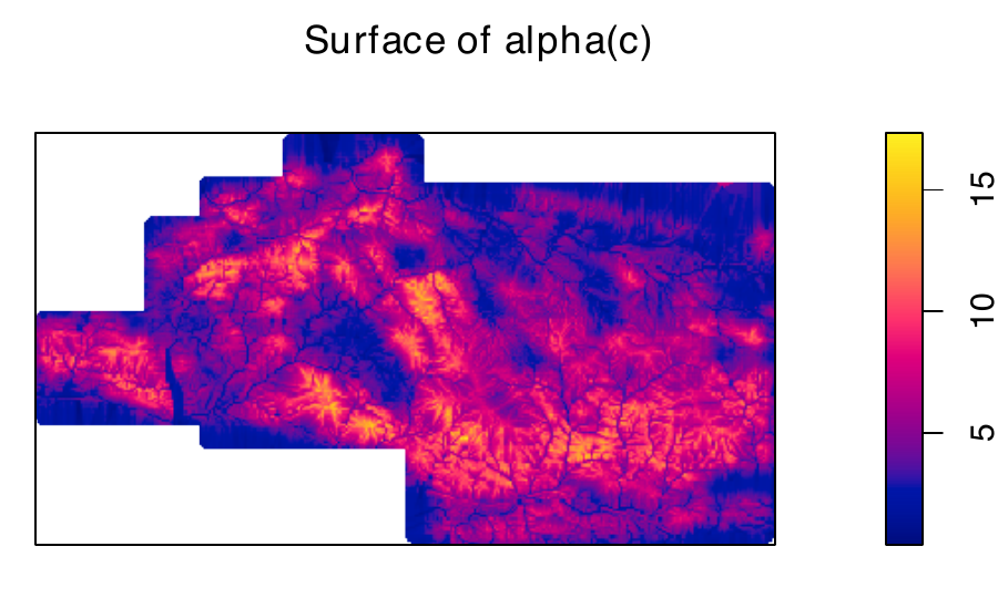
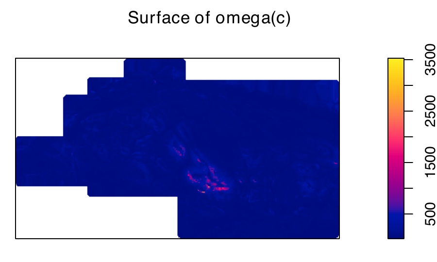
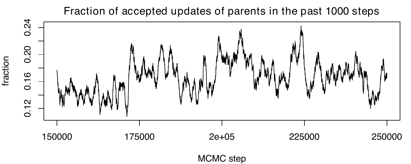
Graphical output, given in Figures 2 to 7, is provided by the command
plot(Output)First, estimated surfaces of the first-order intensity function, the \(\alpha(c)\) function, describing the mean number of points in a cluster, and the \(\omega(c)\) function, describing the spread of the clusters, are plotted, as illustrated in Figure 2. The estimated surfaces are plotted in the dilated window.
Then, histograms describing the estimated posterior distribution of the model parameters are plotted, see Figure 3.
The histograms for the first-order parameters are not plotted, because
the point estimates of \(\beta_1\) and \(\beta_2\) are computed in the first
step under the assumption of Poissonity. But these parameters govern the
inhomogeneity of cluster centers, i.e. their significance should be
computed from cluster centers only. In order to deal with this issue, we
record the centers in every step of the Markov chain and also we record
the significance of the covariates from the list z_beta with respect
to the population of cluster centers in every step of the chain.
Histograms of the corresponding p-values are plotted instead of the
posterior histograms for these parameters, see the bottom part of
Figure 3. This provides more precise inference
about the significance of the covariates influencing the cluster centers
than the outcomes of the first step of estimation, where the ppm
function from the spatstat package is used and where the locations
of the (observed) offsprings may confound the significance of the
covariates with respect to the (unobserved) parent points.
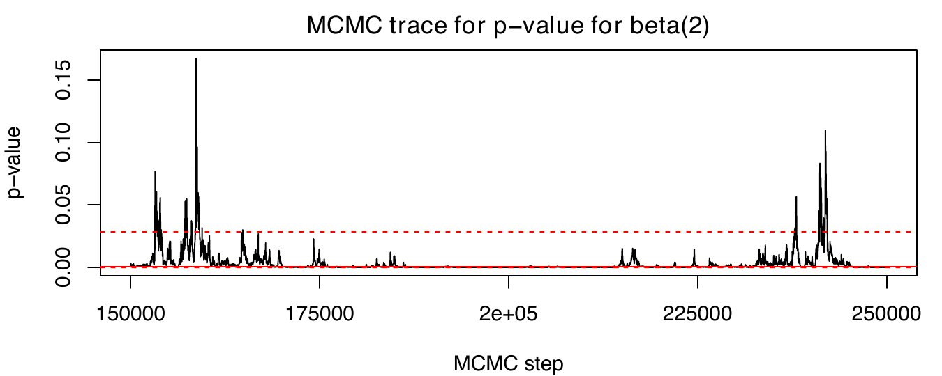
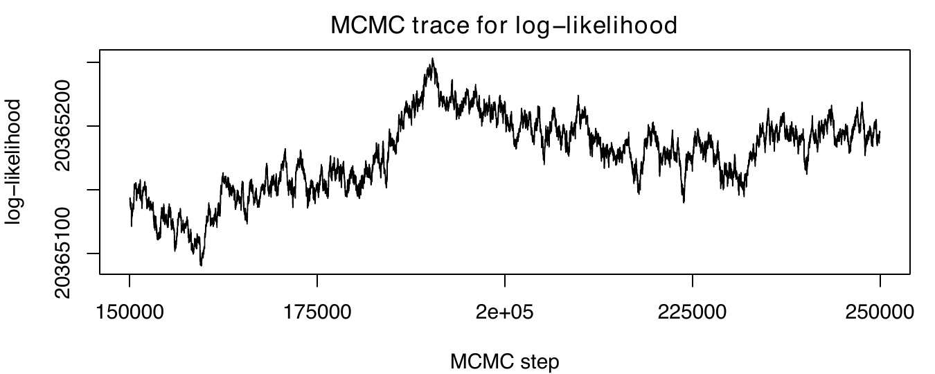
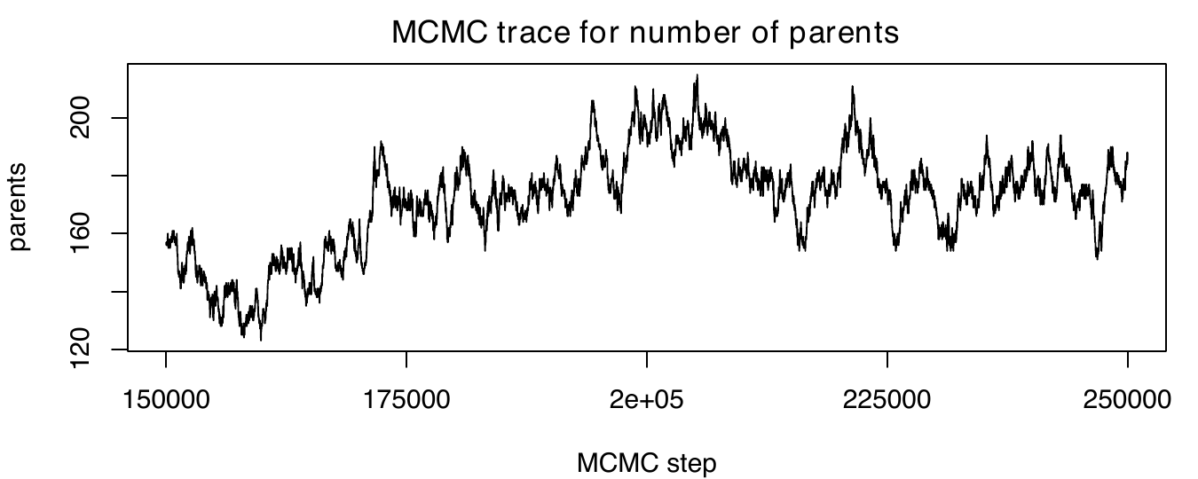
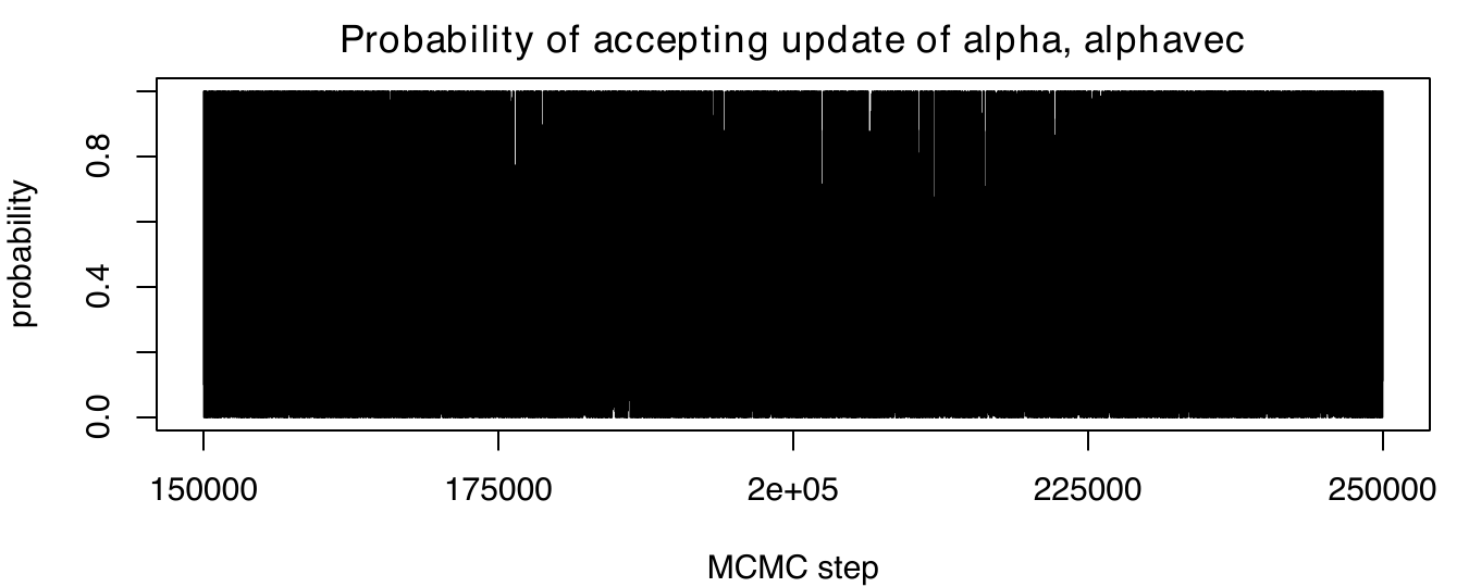
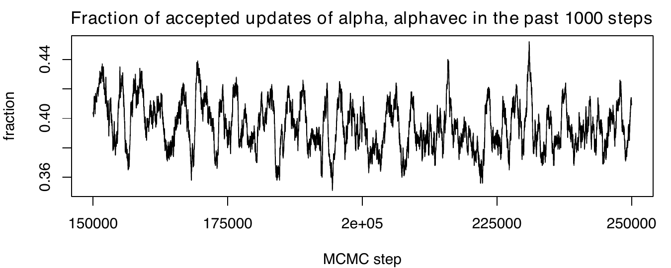
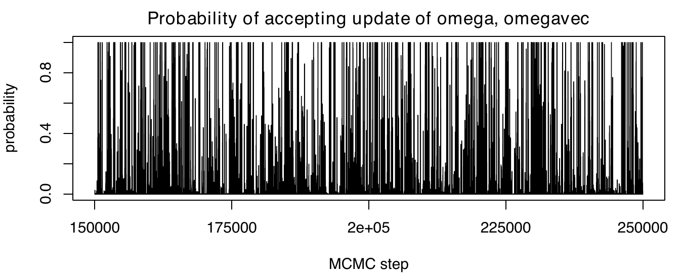
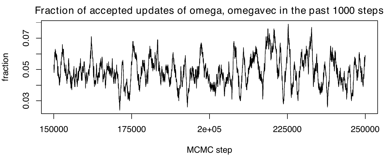
Finally, traceplots for various quantities describing the state of the chain are plotted, including 1) the model parameters, 2) the p-values discussed in the previous paragraph, 3) the value of the log-likelihood itself, 4) the number of parent points in the dilated window, 5) acceptance probabilities for the proposed updates of parameters influencing \(\alpha(c)\) or \(\omega(c)\) (not very informative for long runs but useful when tuning the algorithm for a new dataset with shorter runs), and 6) fractions of accepted updates in the past 1000 steps of the algorithm (much more informative than plots of the acceptance probabilities). See Figures 4 to 7 for illustration. The traceplots for model parameters show also the estimated median of the posterior distribution (given by the solid red line) together with the bounds of the credible interval with the required credibility (red dashed lines). These bounds correspond to the empirical 2.5% and 97.5% quantiles of the posterior distribution when 95% credibility is chosen.
Simulation of the Thomas process with complex inhomogeneity
The Thomas process with any kind of assumed inhomogeneity can be
simulated using the function rThomasInhom. This function generates the
parent process using the rpoispp function from the spatstat
package. The offspring points are simulated directly from the
appropriate normal distributions.
W <- square(1)
W_dil <- dilation.owin(W,0.1)
cov1 <- as.im(function(x,y){x}, W=W_dil)
cov2 <- as.im(function(x,y){y}, W=W_dil)
cov3 <- as.im(function(x,y){1 - (y - 0.5) ^ 2}, W=W_dil)
Y=rThomasInhom(kappa=10, betavec=c(1), z_beta=list(cov1),
             alpha=log(10), alphavec = c(1), z_alpha=list(cov2),
             omega=log(0.01), omegavec=c(1), z_omega=list(cov3),
             W=W, W_dil=W_dil)
Simulation from the fitted model is also possible using the function
simulate.
simulate(Output)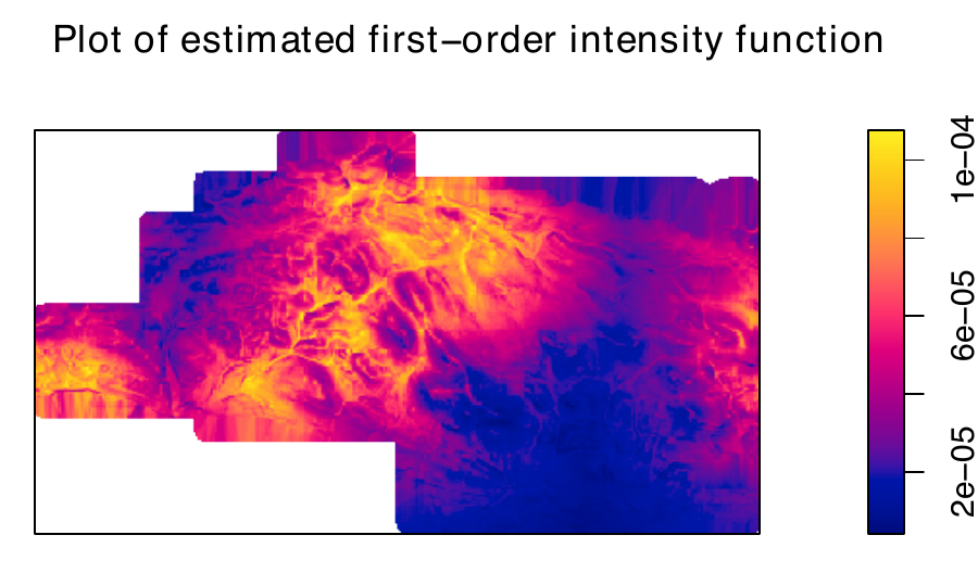
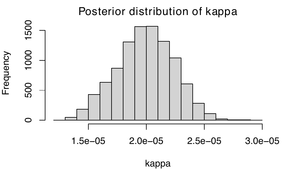
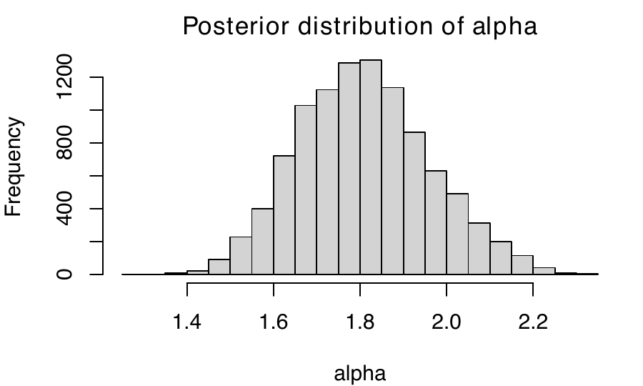
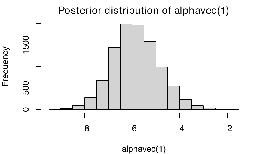
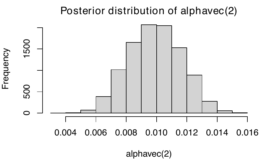
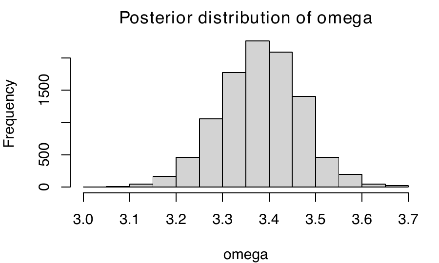
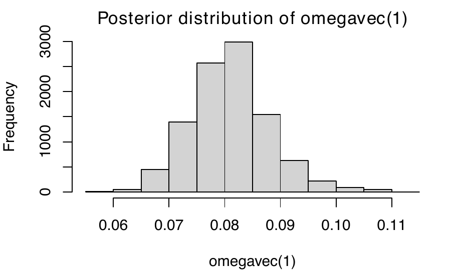
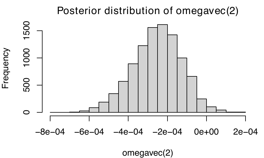
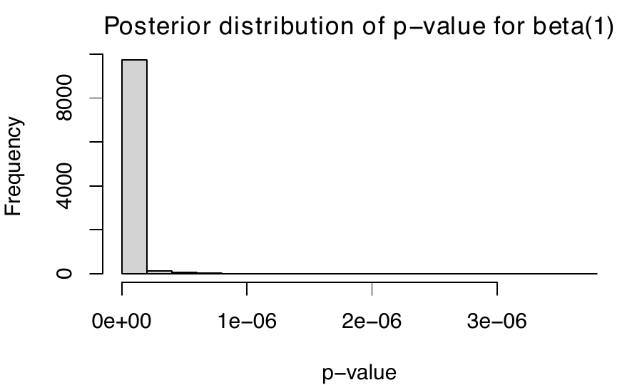
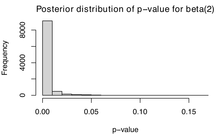
alpha
in the histogram above corresponds to the parameters β0α,
the parameter omega corresponds to β0ω
and the parameters alphavec(i) corresponds to the
parameters βiα
from Section 2, omegavec(i) corresponds to
βiω
and beta(i) corresponds to βi.
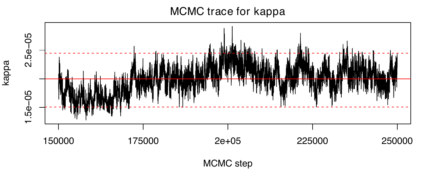
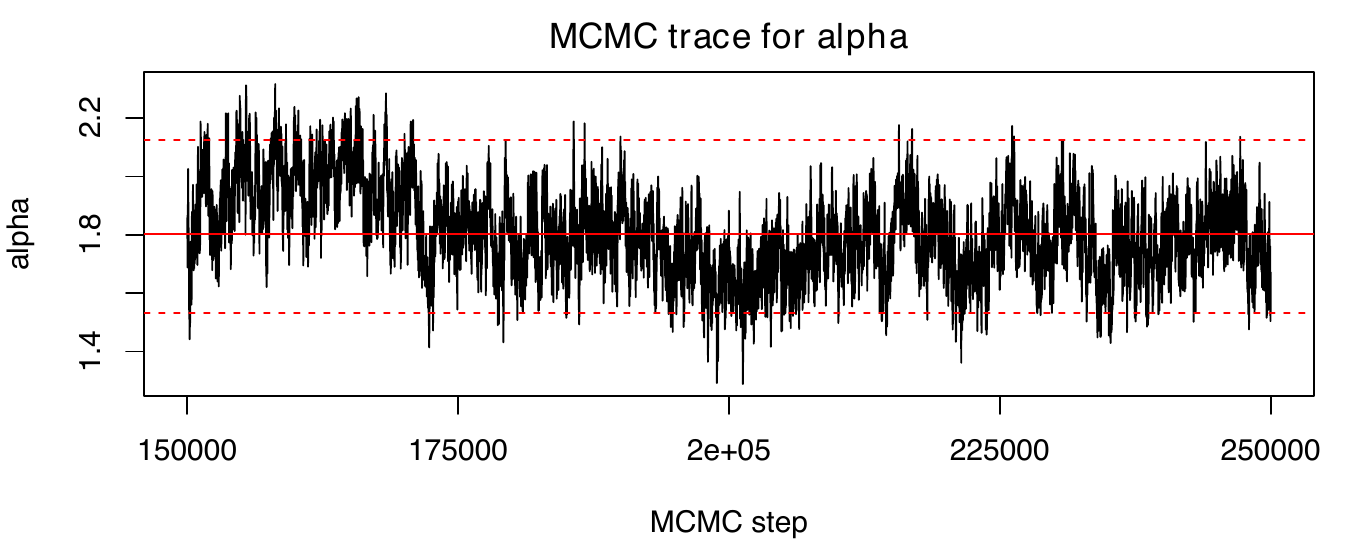
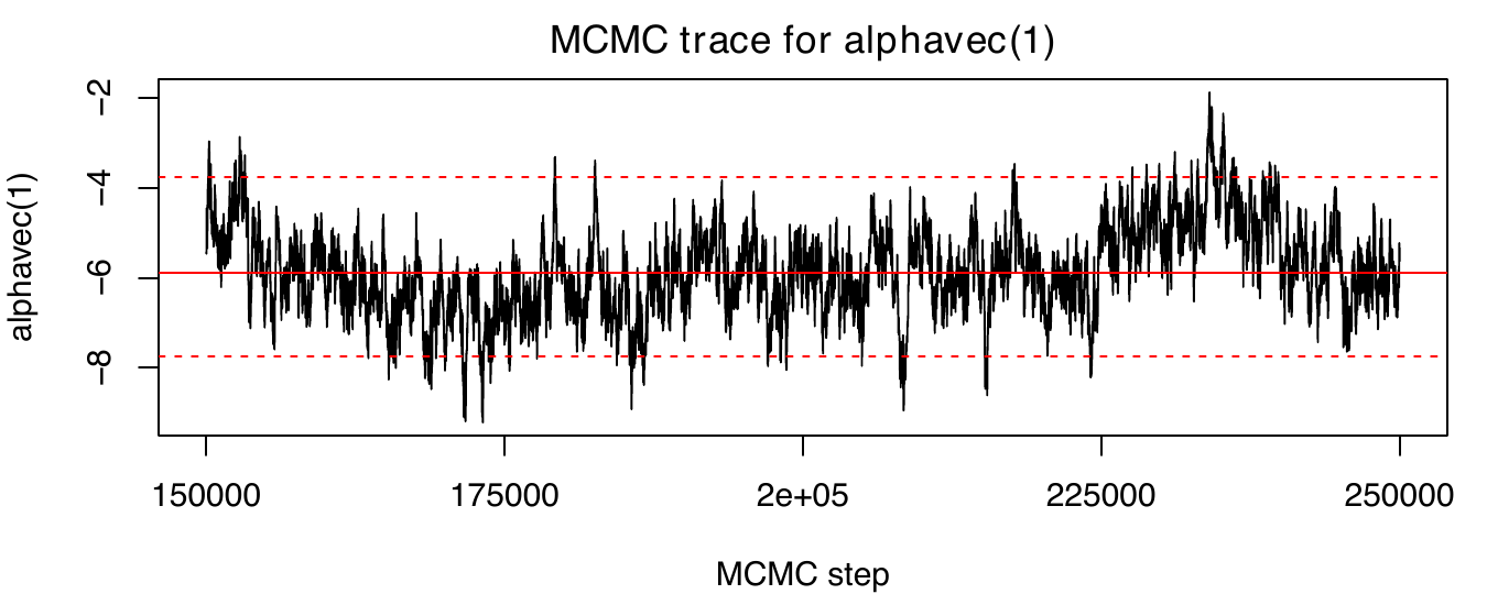
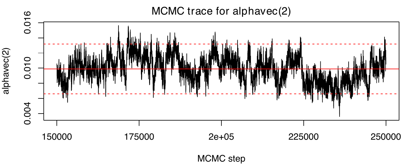
alpha
in the traceplot above corresponds to the parameters β0α
and the parameters alphavec(i) corresponds to the
parameters βiα
from Section 2.2
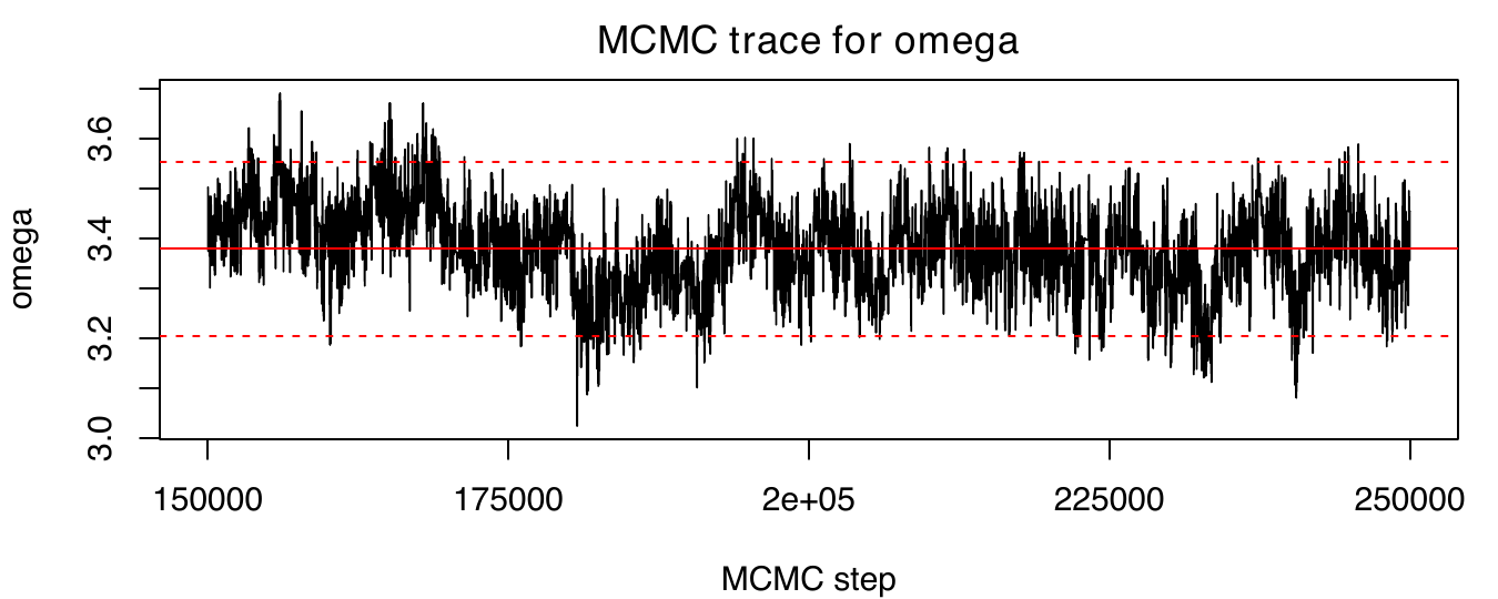
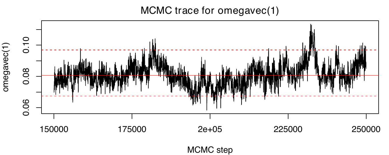
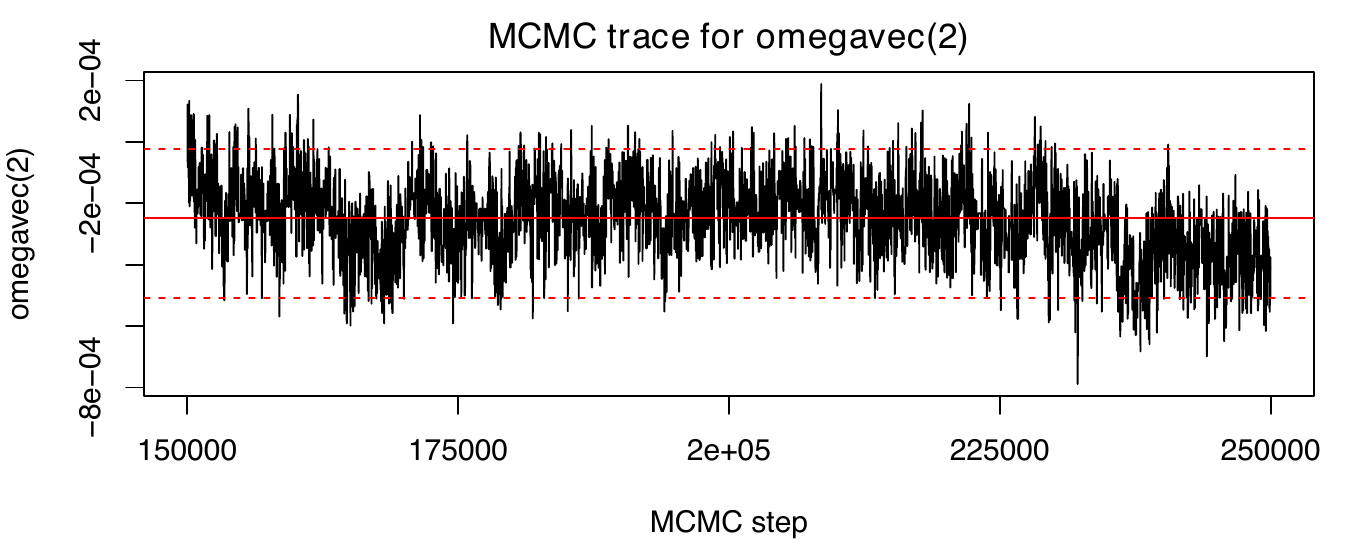
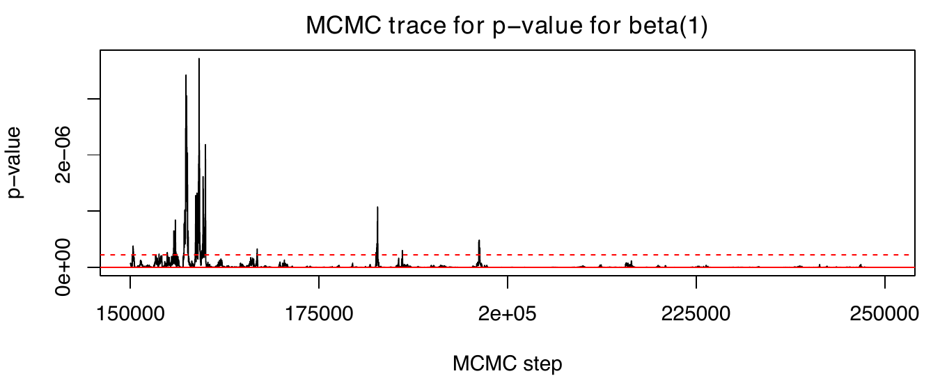
omega corresponds to β0ω
and omegavec(i) corresponds to βiω
and beta(i) corresponds to βi. The
parameter beta(1) corresponds to the β1 computed in the first
step, nevertheless its p-value
is computed in the Bayesian step.
Generalised Neyman-Scott
In this subsection we specify the implementation of the Bayesian MCMC
algorithm for estimation of the homogeneous generalised Thomas point
process (GTPP) which was described in (Andersson and Mrkvička 2020). In
this subsection we assume that the point pattern X is an object of the
format ppp from the spatstat package and that it is observed in a
rectangular observation window W. The notation and priors are slightly
different from those for the inhomogeneous models, due to the different
notations used in the corresponding original papers.
The GTPP can be simulated using
kappa <- 10; omega <- .1; lambda <- .5; theta <- 10
X <- rgtp(kappa, omega, lambda, theta, win = owin(c(0, 1), c(0, 1)))
plot(X$X)
plot(X$C)
Here kappa corresponds to the intensity of centers, omega to the
standard deviation of the radially symmetric Gaussian distribution
determining the spread of offsprings, and lambda and theta
correspond to the parameters of the GPD governing the cluster size.
The priors used in the estimation are lognormal for all parameters,
except lambda which has a uniform prior. The hyperparametres and
control parameters must be specified in the estimation function estgtp
itself. The function estgtpr allows for plotting of all results and
outputs of the MCMC chain.
The posterior distribution of the parameter lambda can be used to
determine the over- or under-dispersion. Specifically, if 0 lies in the
95% credible interval for lambda, then the Poisson assumption cannot
be rejected. See the example code where the result summarizes all
posterior medians and credible intervals for the model parameters.
#Prior for parameter kappa
a_kappa <- 4
b_kappa <- 1
x       <- seq(0, 100, length = 100)
hx      <- dlnorm(x, a_kappa, b_kappa)
plot(x, hx, type = "l", lty = 1, xlab = "x value",
     ylab = "Density", main = "Prior")

#Prior for parameter omega
a_omega <- -3
b_omega <- 1
x       <- seq(0, 1, length = 100)
hx      <- dlnorm(x, a_omega, b_omega)
plot(x, hx, type = "l", lty = 1, xlab = "x value",
     ylab = "Density", main = "Prior")

#Prior for parameter lambda
l_lambda <- -1
u_lambda <- 0.99
x        <- seq(-1, 1, length = 100)
hx       <- dunif(x, l_lambda, u_lambda)
plot(x, hx, type = "l", lty = 1, xlab = "x value",
     ylab = "Density", main = "Prior")

#Prior for parameter theta
a_theta <- 4
b_theta <- 1
x       <- seq(0, 100, length = 100)
hx      <- dlnorm(x, a_theta, b_theta)
plot(x, hx, type = "l", lty = 1, xlab = "x value",
     ylab = "Density", main = "Prior")

#estimation procedure with default values for standard deviations of updates for the parameters
est <- estgtp(X$X,
             skappa = exp(a_kappa + ((b_kappa ^ 2) / 2)) / 100,
             somega = exp(a_omega + ((b_omega ^ 2) / 2)) / 100, dlambda = 0.01,
             stheta = exp(a_theta + ((b_theta ^ 2) / 2)) / 100, smove = 0.1,
             a_kappa = a_kappa, b_kappa = b_kappa,
             a_omega = a_omega, b_omega = b_omega,
             l_lambda = l_lambda, u_lambda = u_lambda,
             a_theta = a_theta, b_theta = b_theta,
             iter = 1000, plot.step = 1000, save.step = 1e9,
             filename = "")

#plotting the results and estimationg of the parameters from refined MCMC chain
discard <- 100
step <- 10

result <- estgtpr(est, discard, step)
result
5 Summary
This paper presents a model and an implementation of the Bayesian MCMC algorithm for estimating parameters of inhomogeneous Neyman-Scott point process with inhomogeneity in cluster centers, cluster spread and/or cluster sizes. The simulation studies assessing the performance of the presented algorithm were published in (Kopecký and Mrkvička 2016) for the homogeneous process, in (Mrkvička et al., 2014) for inhomogeneous cluster centers and in (Mrkvička and Soubeyrand, 2017) for inhomogeneous cluster centers and cluster spread.
The presented package binspp allows also for identification of over- or under-dispersion of cluster sizes in a homogeneous model through the generalised Thomas point process. Since the algorithm is rather flexible, the package can be further extended by estimation methods for models where some cluster centers are given and fixed. It can also be extended in the direction of the spatio-temporal Neyman-Scott point processes.
A user of this package should be aware of the following issues, connected with the Bayesian MCMC algorithms. First, priors should be carefully chosen, even though we provide a sensible default. For example, the range of the \(\omega\) prior must be in coherence with the size of the observation window; similarly, the range of the priors for the regression parameters connected with the covariates must reflect the range of the covariate values. Second, when slow mixing is observed via low fractions of accepted updates, one might think of changing the standard deviation for proposal distributions. These standard deviations are also provided in the package by their default value. Third, if many covariates are considered, longer chains are needed to get reasonably close to the equilibrium. The equilibrium state can be determined by the log-likelihood not increasing anymore, stabilized number of centers, stationary behaviour of the trace plots of the parameters, or by unimodal histograms of posterior distributions.
Acknowledgements
The project has been financially supported by the Grant Agency of Czech Republic (Project No. 19-04412S) and by the ERC CZ grant LL2407 of the Ministry of Education, Youth and Sport of the Czech Republic. The authors wish to express their gratitude to the editor and the anonymous referees for their insightful comments both on the text of the manuscript and the implementation of the package itself. The authors are also grateful to Begona Abellanas who initiated this project by asking for the implementation of the method and who provided the real data set.
6 CRAN packages used
7 CRAN Task Views implied by cited packages
MixedModels, Spatial, SpatioTemporal, Survival
8 Note
This article is converted from a Legacy LaTeX article using the texor package. The pdf version is the official version. To report a problem with the html, refer to CONTRIBUTE on the R Journal homepage.